非官方中文翻译 本页译自 MNE-Python 官方文档： 查看英文原文 ↗。 文档版权归 MNE Developers 所有（BSD-3-Clause）。

跨半球比较

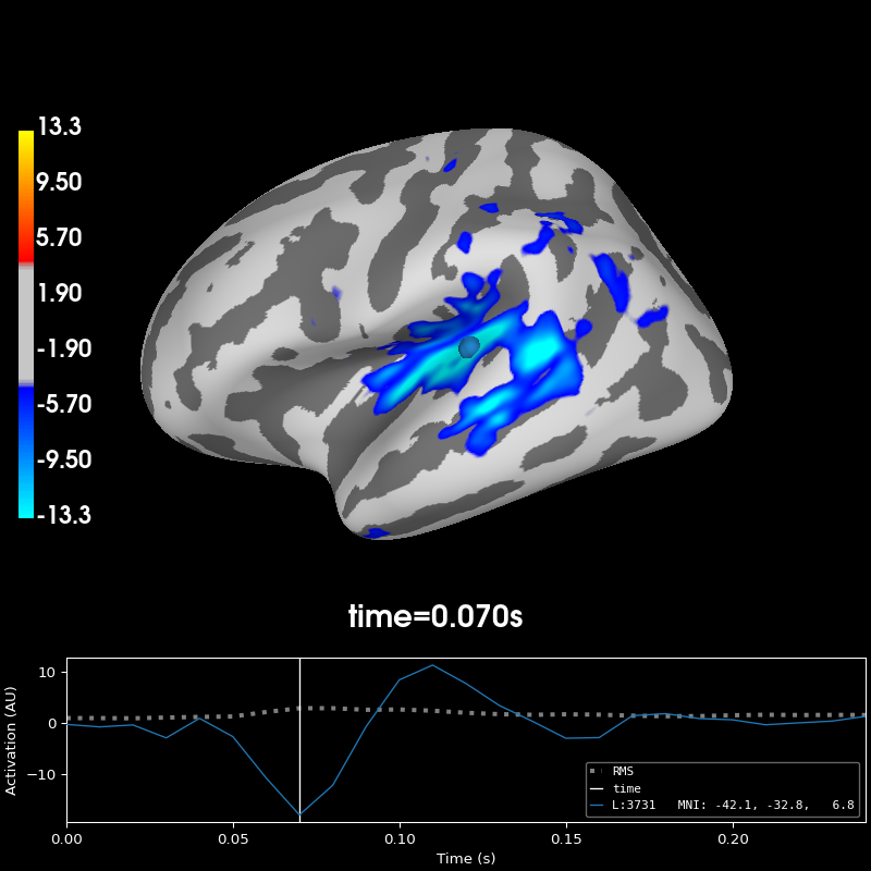
本示例展示如何可视化左右半球活动的差异：把右半球的数据映射到左半球，再绘制二者之差。更多信息参见 mne.compute_source_morph()。

# Author: Christian Brodbeck <christianbrodbeck@nyu.edu>
#
# License: BSD-3-Clause
# Copyright the MNE-Python contributors.

import mne

data_dir = mne.datasets.sample.data_path()
subjects_dir = data_dir / "subjects"
stc_path = data_dir / "MEG" / "sample" / "sample_audvis-meg-eeg"
stc = mne.read_source_estimate(stc_path, "sample")

# First, morph the data to fsaverage_sym, for which we have left_right
# registrations:
stc = mne.compute_source_morph(
    stc, "sample", "fsaverage_sym", smooth=5, warn=False, subjects_dir=subjects_dir
).apply(stc)

# Compute a morph-matrix mapping the right to the left hemisphere,
# and vice-versa.
morph = mne.compute_source_morph(
    stc,
    "fsaverage_sym",
    "fsaverage_sym",
    spacing=stc.vertices,
    warn=False,
    subjects_dir=subjects_dir,
    xhemi=True,
    verbose="error",
)  # creating morph map
stc_xhemi = morph.apply(stc)

# Now we can subtract them and plot the result:
diff = stc - stc_xhemi

diff.plot(hemi="lh", subjects_dir=subjects_dir, initial_time=0.07, size=(800, 600))

surface source space present ...
Computing morph matrix...
    Left-hemisphere map read.
    Right-hemisphere map read.
    5 smooth iterations done.
    5 smooth iterations done.
[done]
[done]
Using control points [ 3.70314401  4.48867635 13.29875944]