
注意
转到末尾下载完整示例代码。
头模型与正向计算#
本教程旨在为正向计算提供一个入门指南。
关于正向建模一般概念更详细的介绍和讲解,请参阅 The forward solution。
# Authors: The MNE-Python contributors.
# License: BSD-3-Clause
# Copyright the MNE-Python contributors.
import mne
from mne.datasets import sample

data_path = sample.data_path()

# the raw file containing the channel location + types
sample_dir = data_path / "MEG" / "sample"
raw_fname = sample_dir / "sample_audvis_raw.fif"

# The paths to FreeSurfer reconstructions
subjects_dir = data_path / "subjects"
subject = "sample"
计算正向算子#
要计算正向算子,我们需要:
一个包含配准信息的
-trans.fif文件。一个源空间
BEM 表面
计算并可视化 BEM 表面#
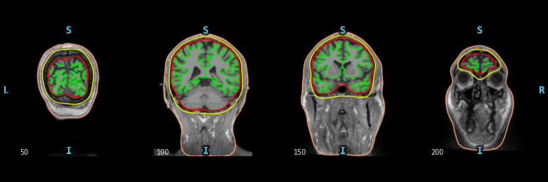
BEM 表面是不同组织之间界面的三角网格剖分,正向计算需要用到它们。这些表面例如包括内颅骨表面、外颅骨表面和外皮肤表面(即头皮表面)。
计算 BEM 表面需要 FreeSurfer,并使用命令行工具 mne watershed_bem 或 mne flash_bem,或相关函数 mne.bem.make_watershed_bem() 或 mne.bem.make_flash_bem()。
这里我们假设它已经计算完成。每位受试者大约需要几分钟。
对于 EEG,我们使用 3 层(内颅骨、外颅骨和皮肤),而对于 MEG,1 层(内颅骨)就足够了。
我们来看一下这些表面。函数 mne.viz.plot_bem() 假定你的受试者 FreeSurfer 重建结果中存在 bem 文件夹,其中包含所需的表面文件。为加快速度,这里我们使用的切片子集比默认值小。
plot_bem_kwargs = dict(
    subject=subject,
    subjects_dir=subjects_dir,
    brain_surfaces="white",
    orientation="coronal",
    slices=[50, 100, 150, 200],
)

mne.viz.plot_bem(**plot_bem_kwargs)
Using surface: /home/circleci/mne_data/MNE-sample-data/subjects/sample/bem/inner_skull.surf
Using surface: /home/circleci/mne_data/MNE-sample-data/subjects/sample/bem/outer_skull.surf
Using surface: /home/circleci/mne_data/MNE-sample-data/subjects/sample/bem/outer_skin.surf
可视化配准#
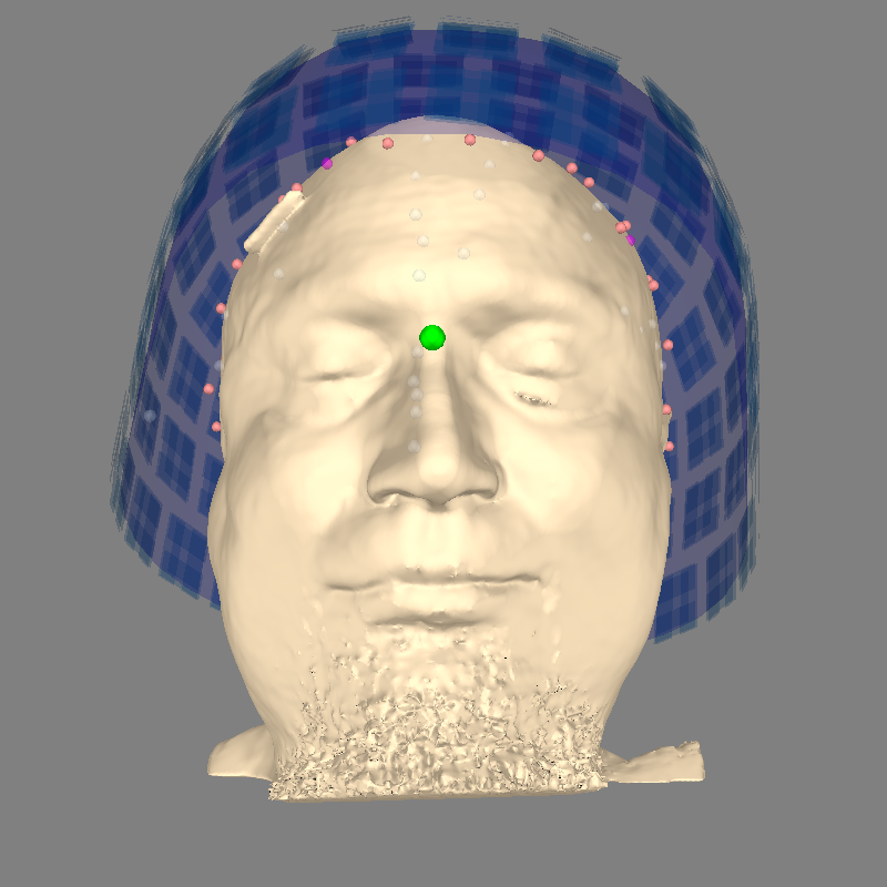
配准(coregistration)是将头部和传感器定位到同一坐标系中的操作。在 MNE 软件中,用于对齐头部和传感器的变换存储在所谓的 trans 文件 中。它是一个以 -trans.fif 结尾的 FIF 文件。可以通过 mne.gui.coregistration()(或其便捷的命令行等价物 mne coreg)获得,若使用 Neuromag 系统也可以使用 mrilab。
这里我们假设配准已经完成,因此只需用下面的代码目视检查对齐情况。关于如何交互式创建 -trans.fif 文件,请参阅 Defining the head↔MRI trans using the GUI。
# The transformation file obtained by coregistration
trans = sample_dir / "sample_audvis_raw-trans.fif"

info = mne.io.read_info(raw_fname)
# Here we look at the dense head, which isn't used for BEM computations but
# is useful for coregistration.
mne.viz.plot_alignment(
    info,
    trans,
    subject=subject,
    dig=True,
    meg=["helmet", "sensors"],
    subjects_dir=subjects_dir,
    surfaces="head-dense",
)
    Read a total of 3 projection items:
        PCA-v1 (1 x 10²)  idle
        PCA-v2 (1 x 10²)  idle
        PCA-v3 (1 x 10²)  idle
Using lh.seghead for head surface.
Getting helmet for system 306m
Channel types:: grad: 203, mag: 102, eeg: 59
计算源空间#
源空间定义了候选源位置的位置和朝向。源空间有两种类型:
基于表面的源空间:候选源被限制在一个表面上。
体积源空间或离散源空间:候选源是被表面包围的离散、任意位置的源点。
基于表面的源空间使用 mne.setup_source_space() 计算,而体积源空间使用 mne.setup_volume_source_space() 计算。
现在我们将计算一个分辨率为 'oct4' 的基于表面的源空间。有关源空间定义和间距参数的详细信息,请参阅 Setting up the source space。
警告
这里使用 'oct4' 只是为了速度;对于实际分析,推荐的间距是 'oct6'。
src = mne.setup_source_space(
    subject, spacing="oct4", add_dist="patch", subjects_dir=subjects_dir
)
print(src)
Setting up the source space with the following parameters:

SUBJECTS_DIR = /home/circleci/mne_data/MNE-sample-data/subjects
Subject      = sample
Surface      = white
Octahedron subdivision grade 4

>>> 1. Creating the source space...

Doing the octahedral vertex picking...
Loading /home/circleci/mne_data/MNE-sample-data/subjects/sample/surf/lh.white...
Mapping lh sample -> oct (4) ...
    Triangle neighbors and vertex normals...
Loading geometry from /home/circleci/mne_data/MNE-sample-data/subjects/sample/surf/lh.sphere...
Setting up the triangulation for the decimated surface...
loaded lh.white 258/155407 selected to source space (oct = 4)

Loading /home/circleci/mne_data/MNE-sample-data/subjects/sample/surf/rh.white...
Mapping rh sample -> oct (4) ...
    Triangle neighbors and vertex normals...
Loading geometry from /home/circleci/mne_data/MNE-sample-data/subjects/sample/surf/rh.sphere...
Setting up the triangulation for the decimated surface...
loaded rh.white 258/156866 selected to source space (oct = 4)

Calculating patch information (limit=0.0 mm)...
    Computing patch statistics...
    Patch information added...
    Computing patch statistics...
    Patch information added...
You are now one step closer to computing the gain matrix
<SourceSpaces: [<surface (lh), n_vertices=155407, n_used=258>, <surface (rh), n_vertices=156866, n_used=258>] MRI (surface RAS) coords, subject 'sample', ~28.7 MiB>
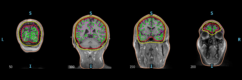
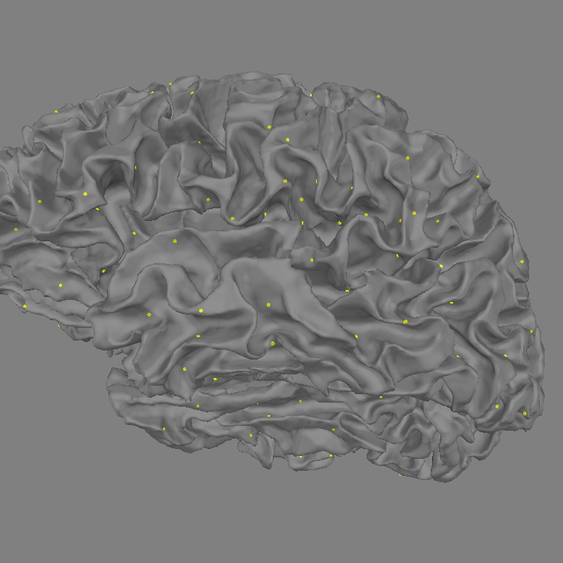
基于表面的源空间 src 包含两部分,一部分对应左半球(258 个位置),另一部分对应右半球(258 个位置)。源可以以紫色显示在 BEM 表面之上。
Using surface: /home/circleci/mne_data/MNE-sample-data/subjects/sample/bem/inner_skull.surf
Using surface: /home/circleci/mne_data/MNE-sample-data/subjects/sample/bem/outer_skull.surf
Using surface: /home/circleci/mne_data/MNE-sample-data/subjects/sample/bem/outer_skin.surf
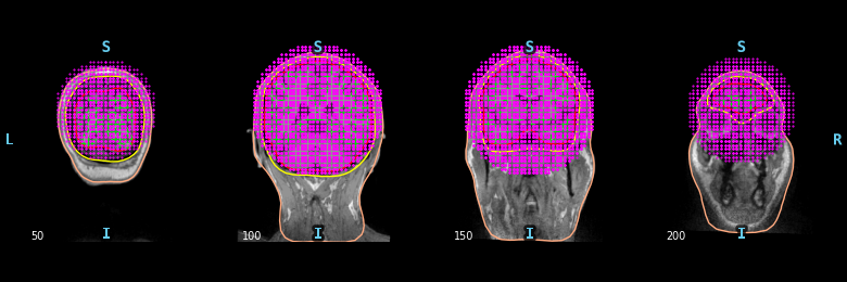
要计算一个体积源空间,其候选偶极子网格位于以 (0.0, 0.0, 40.0) mm 为中心、半径为 90 mm 的球体内,可以使用以下代码。显然,这里的球体并不完美:它并不局限于大脑,可能会遗漏部分皮层。
sphere = (0.0, 0.0, 0.04, 0.09)
vol_src = mne.setup_volume_source_space(
    subject,
    subjects_dir=subjects_dir,
    sphere=sphere,
    sphere_units="m",
    add_interpolator=False,
)  # just for speed!
print(vol_src)

mne.viz.plot_bem(src=vol_src, **plot_bem_kwargs)
Sphere                : origin at (0.0 0.0 40.0) mm
              radius  : 90.0 mm
grid                  : 5.0 mm
mindist               : 5.0 mm
MRI volume            : /home/circleci/mne_data/MNE-sample-data/subjects/sample/mri/T1.mgz

Reading /home/circleci/mne_data/MNE-sample-data/subjects/sample/mri/T1.mgz...

Setting up the sphere...
Surface CM = (   0.0    0.0   40.0) mm
Surface fits inside a sphere with radius   90.0 mm
Surface extent:
    x =  -90.0 ...   90.0 mm
    y =  -90.0 ...   90.0 mm
    z =  -50.0 ...  130.0 mm
Grid extent:
    x =  -95.0 ...   95.0 mm
    y =  -95.0 ...   95.0 mm
    z =  -50.0 ...  135.0 mm
57798 sources before omitting any.
24365 sources after omitting infeasible sources not within 0.0 - 90.0 mm.
Source spaces are in MRI coordinates.
Checking that the sources are inside the surface and at least    5.0 mm away (will take a few...)
    3922 source space point omitted because of the    5.0-mm distance limit.
20443 sources remaining after excluding the sources outside the surface and less than    5.0 mm inside.
Adjusting the neighborhood info.
Source space : MRI voxel -> MRI (surface RAS)
    0.005000 0.000000 0.000000     -95.00 mm
    0.000000 0.005000 0.000000     -95.00 mm
    0.000000 0.000000 0.005000     -50.00 mm
    0.000000 0.000000 0.000000       1.00
MRI volume : MRI voxel -> MRI (surface RAS)
    -0.001000 0.000000 0.000000     128.00 mm
    0.000000 0.000000 0.001000    -128.00 mm
    0.000000 -0.001000 0.000000     128.00 mm
    0.000000 0.000000 0.000000       1.00
MRI volume : MRI (surface RAS) -> RAS (non-zero origin)
    1.000000 -0.000000 -0.000000      -5.27 mm
    -0.000000 1.000000 -0.000000       9.04 mm
    -0.000000 0.000000 1.000000     -27.29 mm
    0.000000 0.000000 0.000000       1.00
<SourceSpaces: [<volume, shape=(np.int64(39), np.int64(39), np.int64(38)), n_used=20443>] MRI (surface RAS) coords, subject 'sample', ~14.3 MiB>
Using surface: /home/circleci/mne_data/MNE-sample-data/subjects/sample/bem/inner_skull.surf
Using surface: /home/circleci/mne_data/MNE-sample-data/subjects/sample/bem/outer_skull.surf
Using surface: /home/circleci/mne_data/MNE-sample-data/subjects/sample/bem/outer_skin.surf
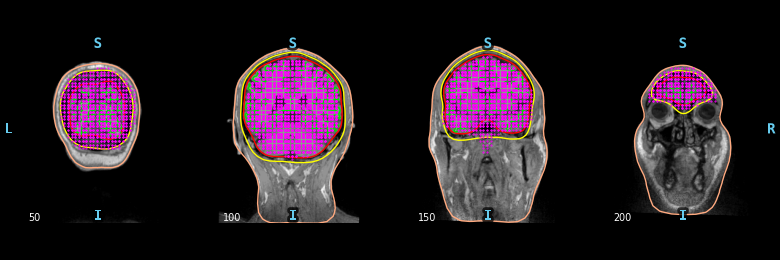
要计算一个体积源空间,其候选偶极子网格位于大脑内部(需要 BEM 表面),可以使用以下代码。
surface = subjects_dir / subject / "bem" / "inner_skull.surf"
vol_src = mne.setup_volume_source_space(
    subject, subjects_dir=subjects_dir, surface=surface, add_interpolator=False
)  # Just for speed!
print(vol_src)

mne.viz.plot_bem(src=vol_src, **plot_bem_kwargs)
Boundary surface file : /home/circleci/mne_data/MNE-sample-data/subjects/sample/bem/inner_skull.surf
grid                  : 5.0 mm
mindist               : 5.0 mm
MRI volume            : /home/circleci/mne_data/MNE-sample-data/subjects/sample/mri/T1.mgz

Reading /home/circleci/mne_data/MNE-sample-data/subjects/sample/mri/T1.mgz...

Loaded bounding surface from /home/circleci/mne_data/MNE-sample-data/subjects/sample/bem/inner_skull.surf (2562 nodes)
Surface CM = (   0.7  -10.0   44.3) mm
Surface fits inside a sphere with radius   91.8 mm
Surface extent:
    x =  -66.7 ...   68.8 mm
    y =  -88.0 ...   79.0 mm
    z =  -44.5 ...  105.8 mm
Grid extent:
    x =  -70.0 ...   70.0 mm
    y =  -90.0 ...   80.0 mm
    z =  -45.0 ...  110.0 mm
32480 sources before omitting any.
22941 sources after omitting infeasible sources not within 0.0 - 91.8 mm.
Source spaces are in MRI coordinates.
Checking that the sources are inside the surface and at least    5.0 mm away (will take a few...)
Checking surface interior status for 22941 points...
    Found  2787/22941 points inside  an interior sphere of radius   43.6 mm
    Found     0/22941 points outside an exterior sphere of radius   91.8 mm
    Found  9357/20154 points outside using surface Qhull
    Found   846/10797 points outside using solid angles
    Total 12738/22941 points inside the surface
Interior check completed in 834.1 ms
    10203 source space points omitted because they are outside the inner skull surface.
    2362 source space points omitted because of the    5.0-mm distance limit.
10376 sources remaining after excluding the sources outside the surface and less than    5.0 mm inside.
Adjusting the neighborhood info.
Source space : MRI voxel -> MRI (surface RAS)
    0.005000 0.000000 0.000000     -70.00 mm
    0.000000 0.005000 0.000000     -90.00 mm
    0.000000 0.000000 0.005000     -45.00 mm
    0.000000 0.000000 0.000000       1.00
MRI volume : MRI voxel -> MRI (surface RAS)
    -0.001000 0.000000 0.000000     128.00 mm
    0.000000 0.000000 0.001000    -128.00 mm
    0.000000 -0.001000 0.000000     128.00 mm
    0.000000 0.000000 0.000000       1.00
MRI volume : MRI (surface RAS) -> RAS (non-zero origin)
    1.000000 -0.000000 -0.000000      -5.27 mm
    -0.000000 1.000000 -0.000000       9.04 mm
    -0.000000 0.000000 1.000000     -27.29 mm
    0.000000 0.000000 0.000000       1.00
<SourceSpaces: [<volume, shape=(np.int64(29), np.int64(35), np.int64(32)), n_used=10376>] MRI (surface RAS) coords, subject 'sample', ~8.0 MiB>
Using surface: /home/circleci/mne_data/MNE-sample-data/subjects/sample/bem/inner_skull.surf
Using surface: /home/circleci/mne_data/MNE-sample-data/subjects/sample/bem/outer_skull.surf
Using surface: /home/circleci/mne_data/MNE-sample-data/subjects/sample/bem/outer_skin.surf
注意
某些源可能看起来位于 BEM 内颅骨轮廓之外。这是因为此处绘图时对切片进行了抽稀。图中的每个切片实际上代表多个 MRI 切片,但只显示单个切片(给定切片范围的中点)的 MRI 体素和 BEM 边界,而绘制在该中点切片上的源空间点则包含所有以该切片(在所显示的所有切片中)为最近切片的点。
现在我们来看看如何在 3D 中查看所有源。
fig = mne.viz.plot_alignment(
    subject=subject,
    subjects_dir=subjects_dir,
    surfaces="white",
    coord_frame="mri",
    src=src,
)
mne.viz.set_3d_view(
    fig,
    azimuth=173.78,
    elevation=101.75,
    distance=0.30,
    focalpoint=(-0.03, -0.01, 0.03),
)
计算正向解#
现在我们可以计算正向解。为减少计算量,我们只计算单层 BEM(仅内颅骨),之后可用于 MEG(而非 EEG)。我们通过 conductivity 参数指定使用单层还是三层 BEM。BEM 解需要一个 BEM 模型,它描述头部的几何结构以及不同组织的电导率。
conductivity = (0.3,)  # for single layer
# conductivity = (0.3, 0.006, 0.3)  # for three layers
model = mne.make_bem_model(
    subject="sample", ico=4, conductivity=conductivity, subjects_dir=subjects_dir
)
bem = mne.make_bem_solution(model)
Creating the BEM geometry...
Going from 4th to 4th subdivision of an icosahedron (n_tri: 5120 -> 5120)
inner skull CM is   0.67 -10.01  44.26 mm
Surfaces passed the basic topology checks.
Complete.

Homogeneous model surface loaded.
Computing the linear collocation solution...
    Matrix coefficients...
        inner skull (2562) -> inner skull (2562) ...
    Inverting the coefficient matrix...
Solution ready.
BEM geometry computations complete.
请注意,BEM 不涉及 trans 文件的使用。BEM 只取决于头部几何结构和电导率,因此它独立于 MEG 数据和头部位置。
现在让我们计算正向算子,通常称为增益矩阵或导联场矩阵。关于每个参数含义的详细信息,请参阅 mne.make_forward_solution()。
Source space          : <SourceSpaces: [<surface (lh), n_vertices=155407, n_used=258>, <surface (rh), n_vertices=156866, n_used=258>] MRI (surface RAS) coords, subject 'sample', ~28.7 MiB>
MRI -> head transform : /home/circleci/mne_data/MNE-sample-data/MEG/sample/sample_audvis_raw-trans.fif
Measurement data      : sample_audvis_raw.fif
Conductor model   : instance of ConductorModel
Accurate field computations
Do computations in head coordinates
Free source orientations

Read 2 source spaces a total of 516 active source locations

Coordinate transformation: MRI (surface RAS) -> head
    0.999310 0.009985 -0.035787      -3.17 mm
    0.012759 0.812405 0.582954       6.86 mm
    0.034894 -0.583008 0.811716      28.88 mm
    0.000000 0.000000 0.000000       1.00

Read 306 MEG channels from info
105 coil definitions read
Coordinate transformation: MEG device -> head
    0.991420 -0.039936 -0.124467      -6.13 mm
    0.060661 0.984012 0.167456       0.06 mm
    0.115790 -0.173570 0.977991      64.74 mm
    0.000000 0.000000 0.000000       1.00
MEG coil definitions created in head coordinates.
Source spaces are now in head coordinates.

Employing the head->MRI coordinate transform with the BEM model.
BEM model instance of ConductorModel is now set up


Source spaces are in head coordinates.
Checking that the sources are inside the surface and at least    5.0 mm away (will take a few...)
Checking surface interior status for 258 points...
    Found  54/258 points inside  an interior sphere of radius   43.6 mm
    Found   0/258 points outside an exterior sphere of radius   91.8 mm
    Found   0/204 points outside using surface Qhull
    Found   0/204 points outside using solid angles
    Total 258/258 points inside the surface
Interior check completed in 14.4 ms
    23 source space point omitted because of the    5.0-mm distance limit.
    Computing patch statistics...
    Patch information added...
Checking surface interior status for 258 points...
    Found  51/258 points inside  an interior sphere of radius   43.6 mm
    Found   0/258 points outside an exterior sphere of radius   91.8 mm
    Found   0/207 points outside using surface Qhull
    Found   0/207 points outside using solid angles
    Total 258/258 points inside the surface
Interior check completed in 16.6 ms
    19 source space point omitted because of the    5.0-mm distance limit.
    Computing patch statistics...
    Patch information added...
Checking surface interior status for 306 points...
    Found   0/306 points inside  an interior sphere of radius   43.6 mm
    Found 306/306 points outside an exterior sphere of radius   91.8 mm
    Found   0/  0 points outside using surface Qhull
    Found   0/  0 points outside using solid angles
    Total 0/306 points inside the surface
Interior check completed in 0.5 ms

Composing the field computation matrix...
Computing MEG at 474 source locations (free orientations)...

Finished.
<Forward | MEG channels: 306 | EEG channels: 0 | Source space: Surface with 474 vertices | Source orientation: Free>
警告
正向计算可能会移除距离内颅骨表面太近(或在其外部)的顶点。例如,这里使用的顶点从 516 个减少到 474 个。对于许多函数(如 mne.compute_source_morph()),重要的是传入 fwd['src'] 或 inv['src'],以便正确地考虑这种移除。
Before: <SourceSpaces: [<surface (lh), n_vertices=155407, n_used=258>, <surface (rh), n_vertices=156866, n_used=258>] MRI (surface RAS) coords, subject 'sample', ~28.7 MiB>
After:  <SourceSpaces: [<surface (lh), n_vertices=155407, n_used=235>, <surface (rh), n_vertices=156866, n_used=239>] head coords, subject 'sample', ~28.7 MiB>
我们可以查看 fwd 的内容,以访问包含增益矩阵的 numpy 数组。
leadfield = fwd["sol"]["data"]
print(f"Leadfield size : {leadfield.shape[0]} sensors x {leadfield.shape[1]} dipoles")
Leadfield size : 306 sensors x 1422 dipoles
要提取对应于源空间 fwd['src'] 且带皮层朝向约束的正向算子所对应的 numpy 数组,可以使用以下代码:
fwd_fixed = mne.convert_forward_solution(
    fwd, surf_ori=True, force_fixed=True, use_cps=True
)
leadfield = fwd_fixed["sol"]["data"]
print(f"Leadfield size : {leadfield.shape[0]} sensors x {leadfield.shape[1]} dipoles")
    Average patch normals will be employed in the rotation to the local surface coordinates....
    Converting to surface-based source orientations...
    [done]
Leadfield size : 306 sensors x 474 dipoles
这等价于以下代码,它显式地将正向算子应用于由单位算子构成的源估计(此处省略,因为它占用大量内存):
>>> import numpy as np
>>> n_dipoles = leadfield.shape[1]
>>> vertices = [src_hemi['vertno'] for src_hemi in fwd_fixed['src']]
>>> stc = mne.SourceEstimate(1e-9 * np.eye(n_dipoles), vertices)
>>> leadfield = mne.apply_forward(fwd_fixed, stc, info).data / 1e-9
要将正向解保存到磁盘,可以使用 mne.write_forward_solution();要从磁盘读回,可以使用 mne.read_forward_solution()。别忘了,包含正向解的 FIF 文件应以 -fwd.fif 结尾。
要获得固定朝向的正向解,可使用 mne.convert_forward_solution() 将自由朝向的解转换为(表面朝向的)固定朝向。
练习#
通过查看 Display sensitivity maps for EEG and MEG sensors 中绘制的 EEG 灵敏度图并与 MEG 比较,你能论证以下说法吗:
MEG 对径向源不敏感
EEG 对深部源更敏感
如果使用自由朝向而非固定/表面朝向,MEG 灵敏度图和直方图会如何变化?
尝试相应地更改 mne.sensitivity_map() 中的 mode 参数。为什么我们在脑回上看不到任何偶极子?
脚本总运行时间:(0 分钟 17.409 秒)