
非官方中文翻译
本页译自 MNE-Python 官方文档:
查看英文原文 ↗。
文档版权归 MNE Developers 所有(BSD-3-Clause)。
说明
转到末尾下载完整示例代码。
用点扩散污染已知信号#
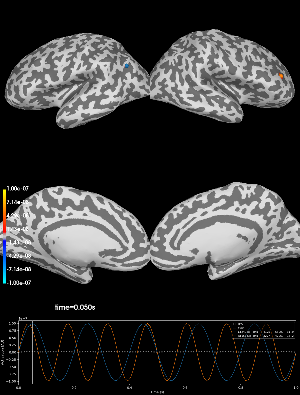
本教程旨在演示如何将已知信号放置在 mne.SourceEstimate 中期望的位置,然后通过应用正向解和逆向解,使该信号因点扩散而受到污染。
# Authors: The MNE-Python contributors.
# License: BSD-3-Clause
# Copyright the MNE-Python contributors.
import numpy as np

import mne
from mne.datasets import sample
from mne.minimum_norm import apply_inverse, read_inverse_operator
from mne.simulation import simulate_evoked, simulate_stc
首先,我们设置一些参数。
seed = 199

# parameters for inverse method
method = "sLORETA"
snr = 3.0
lambda2 = 1.0 / snr**2

# signal simulation parameters
# do not add extra noise to the known signals
nave = np.inf
T = 100
times = np.linspace(0, 1, T)
dt = times[1] - times[0]

# Paths to MEG data
data_path = sample.data_path()
subjects_dir = data_path / "subjects"
fname_fwd = data_path / "MEG" / "sample" / "sample_audvis-meg-oct-6-fwd.fif"
fname_inv = data_path / "MEG" / "sample" / "sample_audvis-meg-oct-6-meg-fixed-inv.fif"
fname_evoked = data_path / "MEG" / "sample" / "sample_audvis-ave.fif"
加载 MEG 数据#
fwd = mne.read_forward_solution(fname_fwd)
fwd = mne.convert_forward_solution(fwd, force_fixed=True, surf_ori=True, use_cps=False)
fwd["info"]["bads"] = []
inv_op = read_inverse_operator(fname_inv)

raw = mne.io.read_raw_fif(data_path / "MEG" / "sample" / "sample_audvis_raw.fif")
raw.info["bads"] = []
raw.set_eeg_reference(projection=True)
events = mne.find_events(raw)
event_id = {"Auditory/Left": 1, "Auditory/Right": 2}
epochs = mne.Epochs(raw, events, event_id, baseline=(None, 0), preload=True)
evoked = epochs.average()

labels = mne.read_labels_from_annot("sample", subjects_dir=subjects_dir)
label_names = [label.name for label in labels]
n_labels = len(labels)
Reading forward solution from /home/circleci/mne_data/MNE-sample-data/MEG/sample/sample_audvis-meg-oct-6-fwd.fif...
    Reading a source space...
    Computing patch statistics...
    Patch information added...
    Distance information added...
    [done]
    Reading a source space...
    Computing patch statistics...
    Patch information added...
    Distance information added...
    [done]
    2 source spaces read
    Desired named matrix (kind = 3523 (FIFF_MNE_FORWARD_SOLUTION_GRAD)) not available
    Read MEG forward solution (7498 sources, 306 channels, free orientations)
    Source spaces transformed to the forward solution coordinate frame
    Changing to fixed-orientation forward solution with surface-based source orientations...
    [done]
Reading inverse operator decomposition from /home/circleci/mne_data/MNE-sample-data/MEG/sample/sample_audvis-meg-oct-6-meg-fixed-inv.fif...
    Reading inverse operator info...
    [done]
    Reading inverse operator decomposition...
    [done]
    305 x 305 full covariance (kind = 1) found.
    Read a total of 4 projection items:
        PCA-v1 (1 x 10²) active
        PCA-v2 (1 x 10²) active
        PCA-v3 (1 x 10²) active
        Average EEG reference (1 x 60) active
    Noise covariance matrix read.
    7498 x 7498 diagonal covariance (kind = 2) found.
    Source covariance matrix read.
    Did not find the desired covariance matrix (kind = 6)
    7498 x 7498 diagonal covariance (kind = 5) found.
    Depth priors read.
    Did not find the desired covariance matrix (kind = 3)
    Reading a source space...
    Computing patch statistics...
    Patch information added...
    Distance information added...
    [done]
    Reading a source space...
    Computing patch statistics...
    Patch information added...
    Distance information added...
    [done]
    2 source spaces read
    Read a total of 4 projection items:
        PCA-v1 (1 x 10²) active
        PCA-v2 (1 x 10²) active
        PCA-v3 (1 x 10²) active
        Average EEG reference (1 x 60) active
    Source spaces transformed to the inverse solution coordinate frame
Opening raw data file /home/circleci/mne_data/MNE-sample-data/MEG/sample/sample_audvis_raw.fif...
    Read a total of 3 projection items:
        PCA-v1 (1 x 10²)  idle
        PCA-v2 (1 x 10²)  idle
        PCA-v3 (1 x 10²)  idle
    Range : 25800 ... 192599 =     42.956 ...   320.670 secs
Ready.
EEG channel type selected for re-referencing
Adding average EEG reference projection.
1 projection items deactivated
Finding events on: STI 014
320 events found on stim channel STI 014
Event IDs: [ 1  2  3  4  5 32]
Not setting metadata
145 matching events found
Setting baseline interval to [-0.19979521315838786, 0.0] s
Applying baseline correction (mode: mean)
Created an SSP operator (subspace dimension = 4)
4 projection items activated
Loading data for 145 events and 421 original time points ...
0 bad epochs dropped
Reading labels from parcellation...
   read 34 labels from /home/circleci/mne_data/MNE-sample-data/subjects/sample/label/lh.aparc.annot
   read 34 labels from /home/circleci/mne_data/MNE-sample-data/subjects/sample/label/rh.aparc.annot
从基线期估计背景噪声协方差#
cov = mne.compute_covariance(epochs, tmin=None, tmax=0.0)
    Created an SSP operator (subspace dimension = 4)
    Setting small MEG eigenvalues to zero (without PCA)
    Setting small EEG eigenvalues to zero (without PCA)
Reducing data rank from 366 -> 362
Estimating covariance using EMPIRICAL
Done.
Number of samples used : 17545
[done]
在空间上相距较远的两个标签中生成正弦信号#
# The known signal is all zero-s off of the two labels of interest
signal = np.zeros((n_labels, T))
idx = label_names.index("inferiorparietal-lh")
signal[idx, :] = 1e-7 * np.sin(5 * 2 * np.pi * times)
idx = label_names.index("rostralmiddlefrontal-rh")
signal[idx, :] = 1e-7 * np.sin(7 * 2 * np.pi * times)
找到每个标签在源空间中的中心顶点#
我们希望每个标签中的已知信号仅在中心处活跃。为此,我们为每个标签创建一个掩码,该掩码在中心顶点处为 1,在标签内所有其他顶点处为 0。随后在仿真源空间数据时使用该掩码。
hemi_to_ind = {"lh": 0, "rh": 1}
for i, label in enumerate(labels):
    # The `center_of_mass` function needs labels to have values.
    labels[i].values.fill(1.0)

    # Restrict the eligible vertices to be those on the surface under
    # consideration and within the label.
    surf_vertices = fwd["src"][hemi_to_ind[label.hemi]]["vertno"]
    restrict_verts = np.intersect1d(surf_vertices, label.vertices)
    com = labels[i].center_of_mass(
        subjects_dir=subjects_dir, restrict_vertices=restrict_verts, surf="white"
    )

    # Convert the center of vertex index from surface vertex list to Label's
    # vertex list.
    cent_idx = np.where(label.vertices == com)[0][0]

    # Create a mask with 1 at center vertex and zeros elsewhere.
    labels[i].values.fill(0.0)
    labels[i].values[cent_idx] = 1.0

    # Print some useful information about this vertex and label
    if "transversetemporal" in label.name:
        dist, _ = label.distances_to_outside(subjects_dir=subjects_dir)
        dist = dist[cent_idx]
        area = label.compute_area(subjects_dir=subjects_dir)
        # convert to equivalent circular radius
        r = np.sqrt(area / np.pi)
        print(
            f"{label.name} COM vertex is {dist * 1e3:0.1f} mm from edge "
            f"(label area equivalent to a circle with r={r * 1e3:0.1f} mm)"
        )
    Triangle neighbors and vertex normals...
transversetemporal-lh COM vertex is 7.5 mm from edge (label area equivalent to a circle with r=11.5 mm)
    Triangle neighbors and vertex normals...
transversetemporal-rh COM vertex is 6.8 mm from edge (label area equivalent to a circle with r=10.8 mm)
创建包含已知信号的源空间数据#
使用信号数组和标签掩码(存储在 labels[i].values 中)将已知信号放置到表面顶点上。
绘制原始信号#
请注意,原始信号是高度集中的(点)源。
kwargs = dict(
    subjects_dir=subjects_dir,
    hemi="split",
    smoothing_steps=4,
    time_unit="s",
    initial_time=0.05,
    size=1200,
    views=["lat", "med"],
)
clim = dict(kind="value", pos_lims=[1e-9, 1e-8, 1e-7])
brain_gen = stc_gen.plot(clim=clim, **kwargs)
仿真传感器空间信号#
使用正向解并添加高斯噪声,从已知的源空间信号仿真传感器空间(诱发)数据。噪声量由 nave 控制(值越大表示噪声越小)。
evoked_gen = simulate_evoked(fwd, stc_gen, evoked.info, cov, nave, rng=seed)

# Map the simulated sensor-space data to source-space using the inverse
# operator.
stc_inv = apply_inverse(evoked_gen, inv_op, lambda2, method=method)
Projecting source estimate to sensor space...
[done]
4 projection items deactivated
Created an SSP operator (subspace dimension = 3)
4 projection items activated
SSP projectors applied...
Preparing the inverse operator for use...
    Scaled noise and source covariance from nave = 1 to nave = 1
    Created the regularized inverter
    Created an SSP operator (subspace dimension = 3)
    Created the whitener using a noise covariance matrix with rank 302 (3 small eigenvalues omitted)
    Computing noise-normalization factors (sLORETA)...
[done]
Applying inverse operator to ""...
    Picked 305 channels from the data
    Computing inverse...
    Eigenleads need to be weighted ...
    Computing residual...
    Explained  99.7% variance
    sLORETA...
[done]
绘制受污染信号的点扩散#
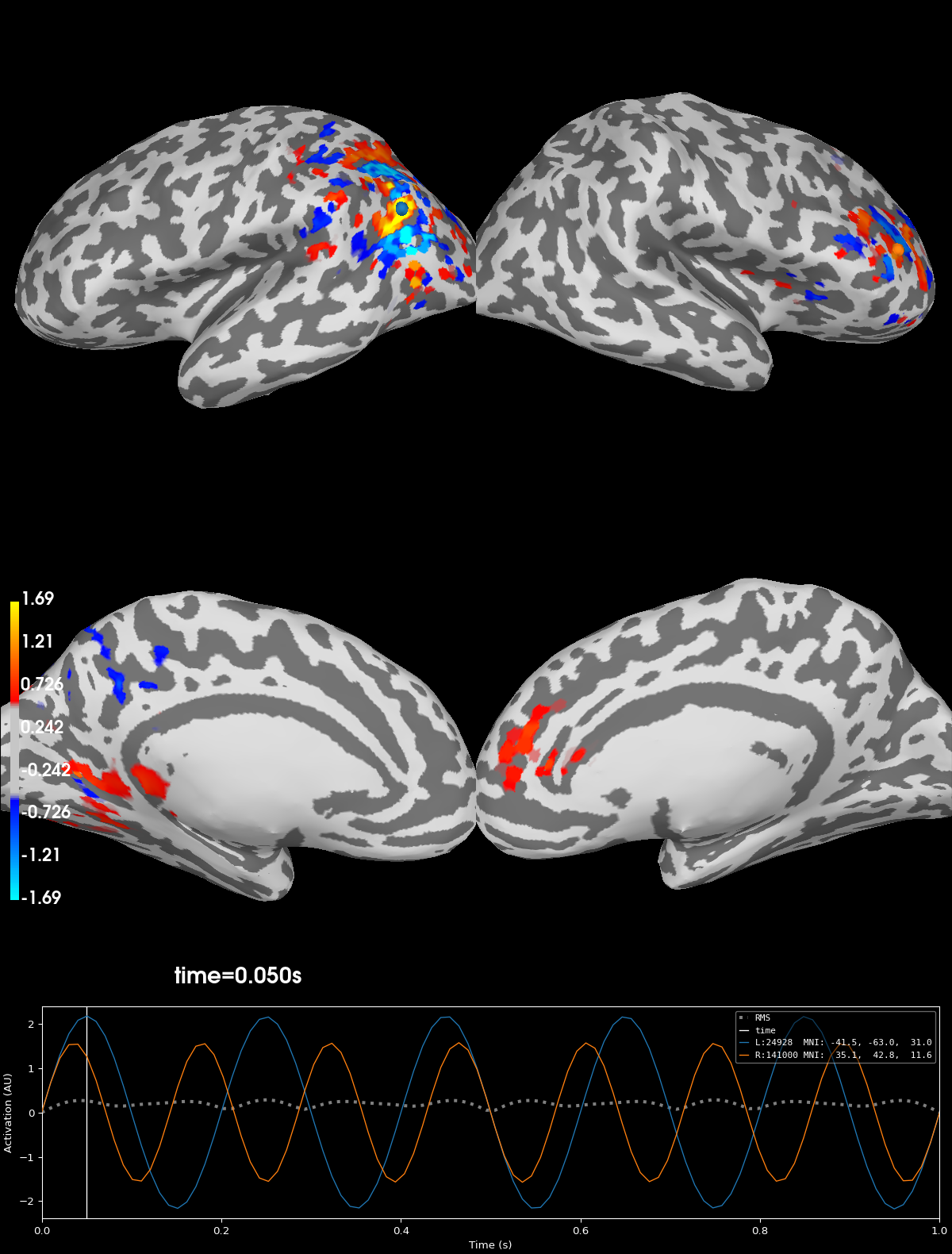
请注意,在将正向算子和逆向算子应用于已知点源之后,点源已在源空间中扩散。这种扩散源于最小范数解,使信号泄漏到方向相近的邻近顶点,因此信号最终会跨越脑沟和脑回。
brain_inv = stc_inv.plot(**kwargs)
Using control points [0.45968308 0.57021267 1.69354621]
练习#
将
method参数改为'dSPM'或'MNE',以探索逆方法的影响。尝试将
evoked_snr设为较小的有限值(例如3.),以观察噪声的影响。
脚本总运行时间:(0 分钟 6.658 秒)