非官方中文翻译 本页译自 MNE-Python 官方文档： 查看英文原文 ↗。 文档版权归 MNE Developers 所有（BSD-3-Clause）。

连续数据的频谱-时间感受野（STRF）估计

本示例演示如何用多个连续输入来拟合编码模型。在这里，我们模拟频谱-时间感受野（STRF）背后的模型。首先，我们创建一个线性滤波器，将频谱-时间空间中的模式映射为表示神经活动的输出。然后，我们拟合一个感受野模型，尝试恢复最初用于生成这些数据的原始线性滤波器。

# Authors: Chris Holdgraf <choldgraf@gmail.com>
#          Eric Larson <larson.eric.d@gmail.com>
#
# License: BSD-3-Clause
# Copyright the MNE-Python contributors.

import matplotlib.pyplot as plt
import numpy as np
from scipy.io import loadmat
from scipy.stats import multivariate_normal
from sklearn.preprocessing import scale

import mne
from mne.decoding import ReceptiveField, TimeDelayingRidge

rng = np.random.default_rng(1337)  # To make this example reproducible

加载音频数据

我们将读取来自 [ 1 ] 的音频数据，以模拟响应。

此外，我们将沿时间维度对数据降采样，以加快计算速度。请注意，根据输入值的不同，这样做可能并不合适。例如，当输入刺激的变化速度比降采样后采样率的一半还快时。

# Read in audio that's been recorded in epochs.
path_audio = mne.datasets.mtrf.data_path()
data = loadmat(str(path_audio / "speech_data.mat"))
audio = data["spectrogram"].T
sfreq = float(data["Fs"][0, 0])
n_decim = 2
audio = mne.filter.resample(audio, down=n_decim, npad="auto")
sfreq /= n_decim

创建感受野

我们将为一个理论上的神经信号模拟线性感受野。它定义了该信号如何对感受野空间中的功率作出响应。

n_freqs = 20
tmin, tmax = -0.1, 0.4

# To simulate the data we'll create explicit delays here
delays_samp = np.arange(np.round(tmin * sfreq), np.round(tmax * sfreq) + 1).astype(int)
delays_sec = delays_samp / sfreq
freqs = np.linspace(50, 5000, n_freqs)
grid = np.array(np.meshgrid(delays_sec, freqs))

# We need data to be shaped as n_epochs, n_features, n_times, so swap axes here
grid = grid.swapaxes(0, -1).swapaxes(0, 1)

# Simulate a temporal receptive field with a Gabor filter
means_high = [0.1, 500]
means_low = [0.2, 2500]
cov = [[0.001, 0], [0, 500000]]
gauss_high = multivariate_normal.pdf(grid, means_high, cov)
gauss_low = -1 * multivariate_normal.pdf(grid, means_low, cov)
weights = gauss_high + gauss_low  # Combine to create the "true" STRF
kwargs = dict(
    vmax=np.abs(weights).max(),
    vmin=-np.abs(weights).max(),
    cmap="RdBu_r",
    shading="gouraud",
)

fig, ax = plt.subplots(layout="constrained")
ax.pcolormesh(delays_sec, freqs, weights, **kwargs)
ax.set(title="Simulated STRF", xlabel="Time Lags (s)", ylabel="Frequency (Hz)")
plt.setp(ax.get_xticklabels(), rotation=45)

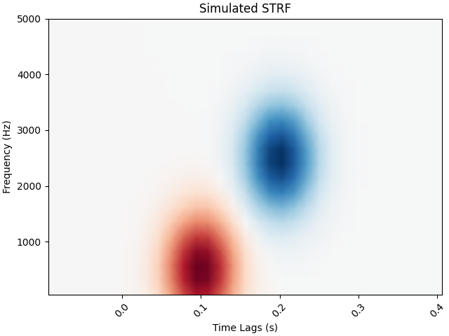
模拟神经响应

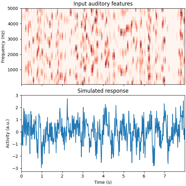
利用这个感受野，我们将生成对刺激的人工神经响应。

为此，我们会创建感受野的时间延迟版本，然后计算它与刺激之间的点积。请注意，这实际上是在刺激与感受野之间进行卷积。更多信息请参见此处。

# Reshape audio to split into epochs, then make epochs the first dimension.
n_epochs, n_seconds = 16, 5
audio = audio[:, : int(n_seconds * sfreq * n_epochs)]
X = audio.reshape([n_freqs, n_epochs, -1]).swapaxes(0, 1)
n_times = X.shape[-1]

# Delay the spectrogram according to delays so it can be combined w/ the STRF
# Lags will now be in axis 1, then we reshape to vectorize
delays = np.arange(np.round(tmin * sfreq), np.round(tmax * sfreq) + 1).astype(int)

# Iterate through indices and append
X_del = np.zeros((len(delays),) + X.shape)
for ii, ix_delay in enumerate(delays):
    # These arrays will take/put particular indices in the data
    take = [slice(None)] * X.ndim
    put = [slice(None)] * X.ndim
    if ix_delay > 0:
        take[-1] = slice(None, -ix_delay)
        put[-1] = slice(ix_delay, None)
    elif ix_delay < 0:
        take[-1] = slice(-ix_delay, None)
        put[-1] = slice(None, ix_delay)
    X_del[ii][tuple(put)] = X[tuple(take)]

# Now set the delayed axis to the 2nd dimension
X_del = np.rollaxis(X_del, 0, 3)
X_del = X_del.reshape([n_epochs, -1, n_times])
n_features = X_del.shape[1]
weights_sim = weights.ravel()

# Simulate a neural response to the sound, given this STRF
y = np.zeros((n_epochs, n_times))
for ii, iep in enumerate(X_del):
    # Simulate this epoch and add random noise
    noise_amp = 0.002
    y[ii] = np.dot(weights_sim, iep) + rng.normal(scale=noise_amp, size=n_times)

# Plot the first 2 trials of audio and the simulated electrode activity
X_plt = scale(np.hstack(X[:2]).T).T
y_plt = scale(np.hstack(y[:2]))
time = np.arange(X_plt.shape[-1]) / sfreq
_, (ax1, ax2) = plt.subplots(2, 1, figsize=(6, 6), sharex=True, layout="constrained")
ax1.pcolormesh(time, freqs, X_plt, vmin=0, vmax=4, cmap="Reds", shading="gouraud")
ax1.set_title("Input auditory features")
ax1.set(ylim=[freqs.min(), freqs.max()], ylabel="Frequency (Hz)")
ax2.plot(time, y_plt)
ax2.set(
    xlim=[time.min(), time.max()],
    title="Simulated response",
    xlabel="Time (s)",
    ylabel="Activity (a.u.)",
)

拟合模型以恢复该感受野

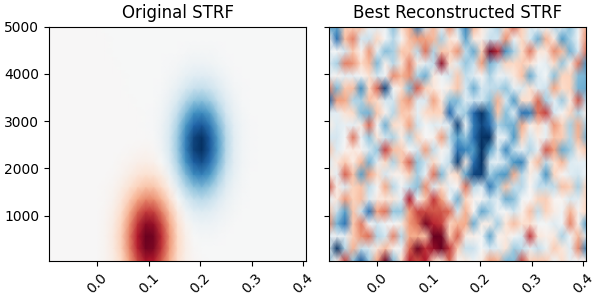
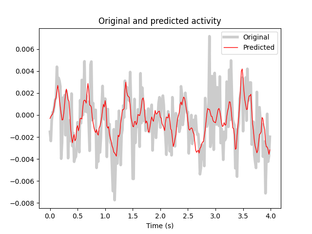
最后，我们将使用 mne.decoding.ReceptiveField 类来恢复该信号的线性感受野。请注意，感受野的性质（例如平滑度）取决于输入与输出的自相关。

# Create training and testing data
train, test = np.arange(n_epochs - 1), n_epochs - 1
X_train, X_test, y_train, y_test = X[train], X[test], y[train], y[test]
X_train, X_test, y_train, y_test = (
    np.rollaxis(ii, -1, 0) for ii in (X_train, X_test, y_train, y_test)
)
# Model the simulated data as a function of the spectrogram input
alphas = np.logspace(-3, 3, 7)
scores = np.zeros_like(alphas)
models = []
for ii, alpha in enumerate(alphas):
    rf = ReceptiveField(tmin, tmax, sfreq, freqs, estimator=alpha)
    rf.fit(X_train, y_train)

    # Now make predictions about the model output, given input stimuli.
    scores[ii] = rf.score(X_test, y_test).item()
    models.append(rf)

times = rf.delays_ / float(rf.sfreq)

# Choose the model that performed best on the held out data
ix_best_alpha = np.argmax(scores)
best_mod = models[ix_best_alpha]
coefs = best_mod.coef_[0]
best_pred = best_mod.predict(X_test)[:, 0]

# Plot the original STRF, and the one that we recovered with modeling.
_, (ax1, ax2) = plt.subplots(
    1,
    2,
    figsize=(6, 3),
    sharey=True,
    sharex=True,
    layout="constrained",
)
ax1.pcolormesh(delays_sec, freqs, weights, **kwargs)
ax2.pcolormesh(times, rf.feature_names, coefs, **kwargs)
ax1.set_title("Original STRF")
ax2.set_title("Best Reconstructed STRF")
plt.setp([iax.get_xticklabels() for iax in [ax1, ax2]], rotation=45)

# Plot the actual response and the predicted response on a held out stimulus
time_pred = np.arange(best_pred.shape[0]) / sfreq
fig, ax = plt.subplots()
ax.plot(time_pred, y_test, color="k", alpha=0.2, lw=4)
ax.plot(time_pred, best_pred, color="r", lw=1)
ax.set(title="Original and predicted activity", xlabel="Time (s)")
ax.legend(["Original", "Predicted"])

• 
• 

Fitting 15 epochs, 20 channels

  0%|          | Sample : 0/3450 [00:00<?,       ?it/s]
  0%|          | Sample : 1/3450 [00:04<4:37:51,    4.83s/it]
 28%|██▊       | Sample : 978/3450 [00:04<00:11,  212.23it/s]
 58%|█████▊    | Sample : 1991/3450 [00:04<00:03,  442.02it/s]
 87%|████████▋ | Sample : 3007/3450 [00:04<00:00,  682.82it/s]Fitting 15 epochs, 20 channels


  0%|          | Sample : 0/3450 [00:00<?,       ?it/s]

 29%|██▉       | Sample : 1003/3450 [00:00<00:00, 62679.90it/s]

 58%|█████▊    | Sample : 2011/3450 [00:00<00:00, 62833.90it/s]

 88%|████████▊ | Sample : 3020/3450 [00:00<00:00, 62913.32it/s]
100%|██████████| Sample : 3450/3450 [00:00<00:00, 62800.43it/s]
Fitting 15 epochs, 20 channels


  0%|          | Sample : 0/3450 [00:00<?,       ?it/s]

 29%|██▉       | Sample : 992/3450 [00:00<00:00, 61991.56it/s]

 58%|█████▊    | Sample : 1992/3450 [00:00<00:00, 62251.74it/s]

 87%|████████▋ | Sample : 3004/3450 [00:00<00:00, 62581.04it/s]
100%|██████████| Sample : 3450/3450 [00:00<00:00, 62523.92it/s]
Fitting 15 epochs, 20 channels


  0%|          | Sample : 0/3450 [00:00<?,       ?it/s]

 29%|██▉       | Sample : 1002/3450 [00:00<00:00, 62617.41it/s]

 59%|█████▊    | Sample : 2019/3450 [00:00<00:00, 63082.70it/s]

 88%|████████▊ | Sample : 3036/3450 [00:00<00:00, 63235.62it/s]
100%|██████████| Sample : 3450/3450 [00:00<00:00, 63171.92it/s]
Fitting 15 epochs, 20 channels


  0%|          | Sample : 0/3450 [00:00<?,       ?it/s]

 29%|██▉       | Sample : 1003/3450 [00:00<00:00, 62631.38it/s]

 59%|█████▊    | Sample : 2022/3450 [00:00<00:00, 63153.38it/s]

 88%|████████▊ | Sample : 3049/3450 [00:00<00:00, 63494.47it/s]
100%|██████████| Sample : 3450/3450 [00:00<00:00, 63500.14it/s]
Fitting 15 epochs, 20 channels


  0%|          | Sample : 0/3450 [00:00<?,       ?it/s]

 29%|██▉       | Sample : 1004/3450 [00:00<00:00, 62703.16it/s]

 59%|█████▊    | Sample : 2020/3450 [00:00<00:00, 63095.19it/s]

 88%|████████▊ | Sample : 3043/3450 [00:00<00:00, 63380.72it/s]
100%|██████████| Sample : 3450/3450 [00:00<00:00, 63352.80it/s]
Fitting 15 epochs, 20 channels


  0%|          | Sample : 0/3450 [00:00<?,       ?it/s]

 29%|██▉       | Sample : 1013/3450 [00:00<00:00, 63293.51it/s]

 59%|█████▉    | Sample : 2045/3450 [00:00<00:00, 63901.32it/s]

 89%|████████▉ | Sample : 3073/3450 [00:00<00:00, 64002.43it/s]
100%|██████████| Sample : 3450/3450 [00:00<00:00, 63900.57it/s]

可视化正则化的效果

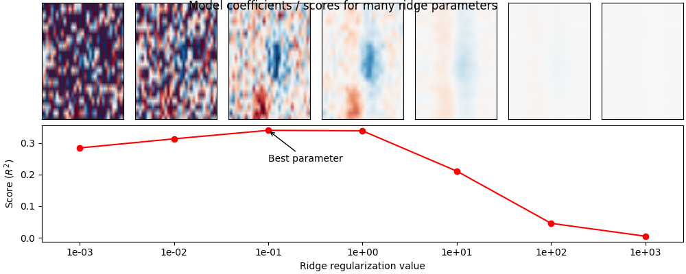
上面我们针对岭正则化参数的众多取值之一，拟合了一个 mne.decoding.ReceptiveField 模型。这里我们将绘制每个取值下的模型得分以及模型系数，以可视化系数如何随正则化程度变化。上述问题以及 STRF 流程在 [ 2 ] [ 3 ] [ 4 ] 中有详细描述。

# Plot model score for each ridge parameter
fig = plt.figure(figsize=(10, 4), layout="constrained")
ax = plt.subplot2grid([2, len(alphas)], [1, 0], 1, len(alphas))
ax.plot(np.arange(len(alphas)), scores, marker="o", color="r")
ax.annotate(
    "Best parameter",
    (ix_best_alpha, scores[ix_best_alpha]),
    (ix_best_alpha, scores[ix_best_alpha] - 0.1),
    arrowprops={"arrowstyle": "->"},
)
plt.xticks(np.arange(len(alphas)), [f"{ii:.0e}" for ii in alphas])
ax.set(
    xlabel="Ridge regularization value",
    ylabel="Score ($R^2$)",
    xlim=[-0.4, len(alphas) - 0.6],
)

# Plot the STRF of each ridge parameter
for ii, (rf, i_alpha) in enumerate(zip(models, alphas)):
    ax = plt.subplot2grid([2, len(alphas)], [0, ii], 1, 1)
    ax.pcolormesh(times, rf.feature_names, rf.coef_[0], **kwargs)
    plt.xticks([], [])
    plt.yticks([], [])
fig.suptitle("Model coefficients / scores for many ridge parameters", y=1)

使用不同的正则化类型

除了标准的岭正则化外，mne.decoding.TimeDelayingRidge 类还提供拉普拉斯正则化项，形式为：

\[\begin{split}\left[\begin{matrix} 1 & -1 & & & & \\ -1 & 2 & -1 & & & \\ & -1 & 2 & -1 & & \\ & & \ddots & \ddots & \ddots & \\ & & & -1 & 2 & -1 \\ & & & & -1 & 1\end{matrix}\right]\end{split}\]

它对相邻的时间采样点和/或特征施加平滑性约束。引用 [ 1 ] 的说法：

Tikhonov [单位] 正则化（公式 5）通过对 TRF 估计进行平滑来减少过拟合，且这种平滑对感兴趣信号的幅度不敏感。然而，拉普拉斯方法（公式 6）在保留信号幅度的同时降低样本外误差（Lalor et al., 2006）。因此，与 Tikhonov 正则化相比，该方法通常能更好地估计系统响应（以 MSE 衡量）。

scores_lap = np.zeros_like(alphas)
models_lap = []
for ii, alpha in enumerate(alphas):
    estimator = TimeDelayingRidge(tmin, tmax, sfreq, reg_type="laplacian", alpha=alpha)
    rf = ReceptiveField(tmin, tmax, sfreq, freqs, estimator=estimator)
    rf.fit(X_train, y_train)

    # Now make predictions about the model output, given input stimuli.
    scores_lap[ii] = rf.score(X_test, y_test).item()
    models_lap.append(rf)

ix_best_alpha_lap = np.argmax(scores_lap)

Fitting 15 epochs, 20 channels


  0%|          | Sample : 0/3450 [00:00<?,       ?it/s]

 30%|██▉       | Sample : 1029/3450 [00:00<00:00, 64255.88it/s]

 60%|█████▉    | Sample : 2069/3450 [00:00<00:00, 64628.86it/s]

 90%|█████████ | Sample : 3107/3450 [00:00<00:00, 64704.26it/s]
100%|██████████| Sample : 3450/3450 [00:00<00:00, 64672.82it/s]
Fitting 15 epochs, 20 channels


  0%|          | Sample : 0/3450 [00:00<?,       ?it/s]

 30%|███       | Sample : 1036/3450 [00:00<00:00, 64720.94it/s]

 60%|██████    | Sample : 2080/3450 [00:00<00:00, 64967.31it/s]

 91%|█████████ | Sample : 3124/3450 [00:00<00:00, 65049.00it/s]
100%|██████████| Sample : 3450/3450 [00:00<00:00, 64962.58it/s]
Fitting 15 epochs, 20 channels


  0%|          | Sample : 0/3450 [00:00<?,       ?it/s]

 30%|███       | Sample : 1040/3450 [00:00<00:00, 64965.99it/s]

 60%|██████    | Sample : 2086/3450 [00:00<00:00, 65152.22it/s]

 91%|█████████ | Sample : 3136/3450 [00:00<00:00, 65312.39it/s]
100%|██████████| Sample : 3450/3450 [00:00<00:00, 65245.82it/s]
Fitting 15 epochs, 20 channels


  0%|          | Sample : 0/3450 [00:00<?,       ?it/s]

 30%|███       | Sample : 1043/3450 [00:00<00:00, 65137.87it/s]

 61%|██████    | Sample : 2095/3450 [00:00<00:00, 65447.10it/s]

 91%|█████████ | Sample : 3146/3450 [00:00<00:00, 65515.57it/s]
100%|██████████| Sample : 3450/3450 [00:00<00:00, 65430.80it/s]
Fitting 15 epochs, 20 channels


  0%|          | Sample : 0/3450 [00:00<?,       ?it/s]

 30%|██▉       | Sample : 1030/3450 [00:00<00:00, 64326.94it/s]

 60%|██████    | Sample : 2081/3450 [00:00<00:00, 64992.57it/s]

 91%|█████████ | Sample : 3126/3450 [00:00<00:00, 65098.16it/s]
100%|██████████| Sample : 3450/3450 [00:00<00:00, 65014.82it/s]
Fitting 15 epochs, 20 channels


  0%|          | Sample : 0/3450 [00:00<?,       ?it/s]

 30%|██▉       | Sample : 1034/3450 [00:00<00:00, 64580.60it/s]

 60%|██████    | Sample : 2080/3450 [00:00<00:00, 64986.79it/s]

 91%|█████████ | Sample : 3125/3450 [00:00<00:00, 65083.23it/s]
100%|██████████| Sample : 3450/3450 [00:00<00:00, 64673.68it/s]
Fitting 15 epochs, 20 channels


  0%|          | Sample : 0/3450 [00:00<?,       ?it/s]

 30%|███       | Sample : 1038/3450 [00:00<00:00, 64838.15it/s]

 60%|██████    | Sample : 2087/3450 [00:00<00:00, 65202.47it/s]

 91%|█████████ | Sample : 3135/3450 [00:00<00:00, 65302.27it/s]
100%|██████████| Sample : 3450/3450 [00:00<00:00, 65230.82it/s]

比较模型性能

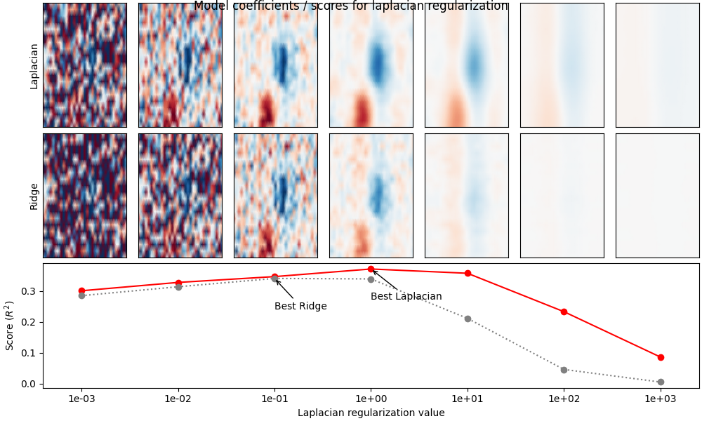
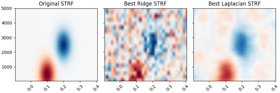
下面我们可视化每种正则化方法（岭回归与拉普拉斯）在不同 alpha 水平下的模型性能。可以看到，拉普拉斯方法通常表现更好，因为它沿系数的维度和特征维度施加平滑性约束。这与“真实”的感受野结构相符，从而获得更好的模型拟合。

fig = plt.figure(figsize=(10, 6), layout="constrained")
ax = plt.subplot2grid([3, len(alphas)], [2, 0], 1, len(alphas))
ax.plot(np.arange(len(alphas)), scores_lap, marker="o", color="r")
ax.plot(np.arange(len(alphas)), scores, marker="o", color="0.5", ls=":")
ax.annotate(
    "Best Laplacian",
    (ix_best_alpha_lap, scores_lap[ix_best_alpha_lap]),
    (ix_best_alpha_lap, scores_lap[ix_best_alpha_lap] - 0.1),
    arrowprops={"arrowstyle": "->"},
)
ax.annotate(
    "Best Ridge",
    (ix_best_alpha, scores[ix_best_alpha]),
    (ix_best_alpha, scores[ix_best_alpha] - 0.1),
    arrowprops={"arrowstyle": "->"},
)
plt.xticks(np.arange(len(alphas)), [f"{ii:.0e}" for ii in alphas])
ax.set(
    xlabel="Laplacian regularization value",
    ylabel="Score ($R^2$)",
    xlim=[-0.4, len(alphas) - 0.6],
)

# Plot the STRF of each ridge parameter
xlim = times[[0, -1]]
for ii, (rf_lap, rf, i_alpha) in enumerate(zip(models_lap, models, alphas)):
    ax = plt.subplot2grid([3, len(alphas)], [0, ii], 1, 1)
    ax.pcolormesh(times, rf_lap.feature_names, rf_lap.coef_[0], **kwargs)
    ax.set(xticks=[], yticks=[], xlim=xlim)
    if ii == 0:
        ax.set(ylabel="Laplacian")
    ax = plt.subplot2grid([3, len(alphas)], [1, ii], 1, 1)
    ax.pcolormesh(times, rf.feature_names, rf.coef_[0], **kwargs)
    ax.set(xticks=[], yticks=[], xlim=xlim)
    if ii == 0:
        ax.set(ylabel="Ridge")
fig.suptitle("Model coefficients / scores for laplacian regularization", y=1)

绘制原始 STRF，以及我们通过建模恢复出的 STRF。

rf = models[ix_best_alpha]
rf_lap = models_lap[ix_best_alpha_lap]
_, (ax1, ax2, ax3) = plt.subplots(
    1,
    3,
    figsize=(9, 3),
    sharey=True,
    sharex=True,
    layout="constrained",
)
ax1.pcolormesh(delays_sec, freqs, weights, **kwargs)
ax2.pcolormesh(times, rf.feature_names, rf.coef_[0], **kwargs)
ax3.pcolormesh(times, rf_lap.feature_names, rf_lap.coef_[0], **kwargs)
ax1.set_title("Original STRF")
ax2.set_title("Best Ridge STRF")
ax3.set_title("Best Laplacian STRF")
plt.setp([iax.get_xticklabels() for iax in [ax1, ax2, ax3]], rotation=45)

参考文献

[1] (1,2)

Michael J. Crosse, Giovanni M. Di Liberto, Adam Bednar, and Edmund C. Lalor. The multivariate temporal response function (mTRF) toolbox: a MATLAB toolbox for relating neural signals to continuous stimuli. Frontiers in Human Neuroscience, 2016. doi:10.3389/fnhum.2016.00604.

[2]

Frédéric E. Theunissen, Stephen V. David, Nandini C. Singh, Ann Hsu, William E. Vinje, and Jack L. Gallant. Estimating spatio-temporal receptive fields of auditory and visual neurons from their responses to natural stimuli. Network: Computation in Neural Systems, 12(3):289–316, 2001. doi:10.1080/net.12.3.289.316.

[3]

Ben Willmore and Darragh Smyth. Methods for first-order kernel estimation: simple-cell receptive fields from responses to natural scenes. Network: Computation in Neural Systems, 14(3):553–577, 2003. doi:10.1088/0954-898X_14_3_309.

[4]

Christopher R. Holdgraf, Wendy de Heer, Brian Pasley, Jochem Rieger, Nathan Crone, Jack J. Lin, Robert T. Knight, and Frédéric E. Theunissen. Rapid tuning shifts in human auditory cortex enhance speech intelligibility. Nature Communications, 2016. doi:10.1038/ncomms13654.