非官方中文翻译本页译自 MNE-Python 官方文档：查看英文原文 ↗。文档版权归 MNE Developers 所有（BSD-3-Clause）。

说明

转到末尾下载完整示例代码。

识别因凝胶过多而短接的 EEG 电极#

科研级 EEG 常使用凝胶系统；凝胶过多时，一个电极从头皮传导信号的凝胶会与另一个电极的凝胶相连，把两个信号“短接”。这很不利，因为两个（或多个）电极的信号不再像本应那样独立，彼此非常相似，带来额外的空间模糊。已有算法可检测电极短接 [1]，并在 EEGLAB 中实现 [2]。遗憾的是，数据采集完成后，除对短接通道插值外，预处理能做的并不多。因此我们建议在数据采集早期检查电极短接并及时处理；若数据已采集完毕，则应量化短接程度，以免该效应给数据引入偏差，并排除短接可能影响研究结论的受试者。预防短接最理想，但至少了解该问题可减轻其作为混杂因素的潜在影响。本教程参照 https://psychophysiology.cpmc.columbia.edu 的 eBridge 教程。

# Authors: Alex Rockhill <aprockhill@mailbox.org>
#
# License: BSD-3-Clause
# Copyright the MNE-Python contributors.

import matplotlib.pyplot as plt
import numpy as np
from matplotlib.colors import LinearSegmentedColormap

import mne

print(__doc__)

计算电距离指标#

首先，我们对 EEGBCI 数据集中一组示例受试者计算电距离指标，以估计电极短接。电距离就是两两相减后信号的方差；活动几乎完全镜像另一通道的通道，其电距离会非常低。通过检查电距离分布，可以寻找始终接近零的成对距离，这提示短接。

说明

通常只需在少量数据（约 3 分钟可能已足够）上运行该算法；但凝胶可能在研究过程中沉降，导致更多短接，因此使用数据最后一段可得到最保守的估计。

montage = mne.channels.make_standard_montage("spherical_1005")
ed_data = dict()  # electrical distance/bridging data
raw_data = dict()  # store infos for electrode positions
for sub in range(1, 11):
    print(f"Computing electrode bridges for subject {sub}")
    raw_fname = mne.datasets.eegbci.load_data(subjects=sub, runs=(1,))[0]
    raw = mne.io.read_raw(raw_fname, preload=True, verbose=False)
    mne.datasets.eegbci.standardize(raw)  # set channel names
    raw.set_montage(montage, verbose=False)
    raw_data[sub] = raw
    ed_data[sub] = mne.preprocessing.compute_bridged_electrodes(raw)

Computing electrode bridges for subject 1
Local minimum 1.1959919512423807e-11 found
Computing electrode bridges for subject 2
Local minimum 7.665886892347756 found
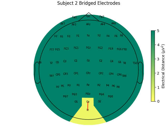
Bridge detected between Oz and Iz
Computing electrode bridges for subject 3
Local minimum 1.1959919512423807e-11 found
Computing electrode bridges for subject 4
Local minimum 3.4367321412134997 found
Bridge detected between FCz and FC2
Bridge detected between FC4 and FC6
Bridge detected between F2 and F4
Computing electrode bridges for subject 5
Local minimum 1.483519741386041e-11 found
Computing electrode bridges for subject 6
Local minimum 4.587817798781012 found
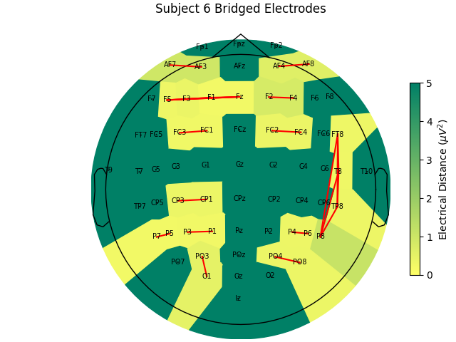
Bridge detected between FC3 and FC1
Bridge detected between FC2 and FC4
Bridge detected between CP3 and CP1
Bridge detected between AF7 and AF3
Bridge detected between AF4 and AF8
Bridge detected between F5 and F3
Bridge detected between F5 and F1
Bridge detected between F5 and Fz
Bridge detected between F3 and F1
Bridge detected between F3 and Fz
Bridge detected between F1 and Fz
Bridge detected between F2 and F4
Bridge detected between FT8 and T8
Bridge detected between FT8 and TP8
Bridge detected between FT8 and P8
Bridge detected between T8 and TP8
Bridge detected between T8 and P8
Bridge detected between TP8 and P8
Bridge detected between P7 and P5
Bridge detected between P3 and P1
Bridge detected between P4 and P6
Bridge detected between PO3 and O1
Bridge detected between PO4 and PO8
Computing electrode bridges for subject 7
Local minimum 9.74600268740129 found
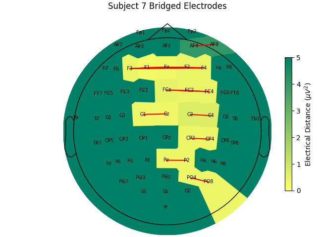
Bridge detected between FCz and FC2
Bridge detected between FCz and FC4
Bridge detected between FC2 and FC4
Bridge detected between C1 and Cz
Bridge detected between C2 and C4
Bridge detected between CP2 and CP4
Bridge detected between AF4 and AF8
Bridge detected between F3 and F1
Bridge detected between F3 and Fz
Bridge detected between F3 and F2
Bridge detected between F3 and F4
Bridge detected between F1 and Fz
Bridge detected between F1 and F2
Bridge detected between F1 and F4
Bridge detected between Fz and F2
Bridge detected between Fz and F4
Bridge detected between F2 and F4
Bridge detected between Pz and P2
Bridge detected between PO4 and PO8
Computing electrode bridges for subject 8
Local minimum 11.590631749462851 found
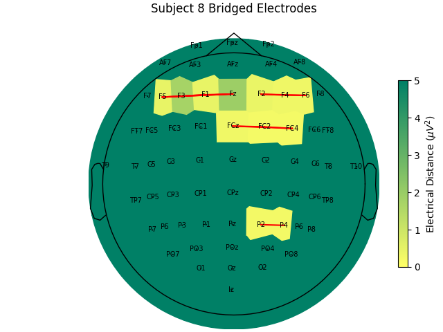
Bridge detected between FCz and FC2
Bridge detected between FCz and FC4
Bridge detected between FC2 and FC4
Bridge detected between F5 and F3
Bridge detected between F5 and F1
Bridge detected between F5 and Fz
Bridge detected between F3 and F1
Bridge detected between F3 and Fz
Bridge detected between F1 and Fz
Bridge detected between F2 and F4
Bridge detected between F2 and F6
Bridge detected between F4 and F6
Bridge detected between P2 and P4
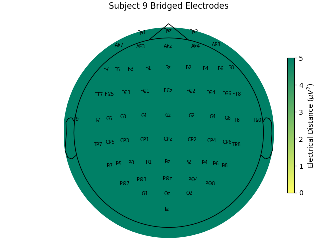
Computing electrode bridges for subject 9
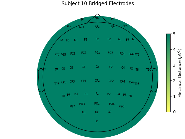
Computing electrode bridges for subject 10

检查电距离矩阵#

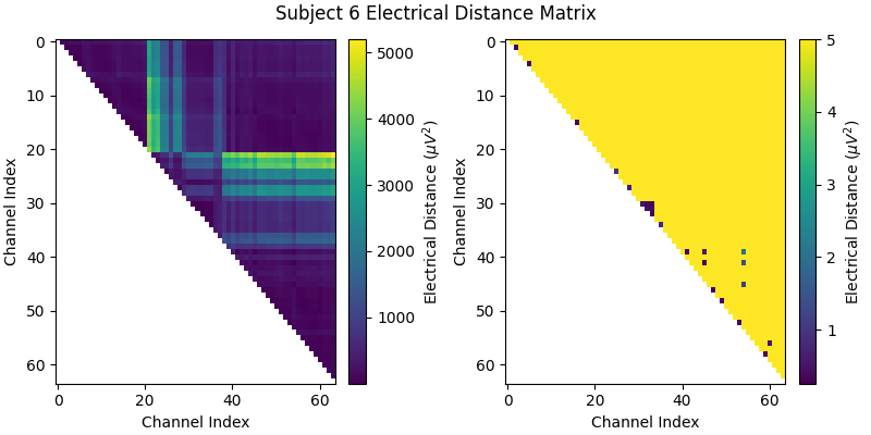
在查看跨受试者的电距离分布之前，先看单个受试者的距离矩阵，理解算法如何工作。我们选受试者 6，它是短接的典型例子。右侧缩小色标范围的版本中可以看到，该受试者的电距离分布与其头部生理/几何结构及记录期间脑活动有关；右侧把色标范围裁剪放大后，可见若干接近零的电距离离群值，提示短接。

bridged_idx, ed_matrix = ed_data[6]

fig, (ax1, ax2) = plt.subplots(1, 2, figsize=(8, 4), layout="constrained")
fig.suptitle("Subject 6 Electrical Distance Matrix")

# take median across epochs, only use upper triangular, lower is NaNs
ed_plot = np.zeros(ed_matrix.shape[1:]) * np.nan
triu_idx = np.triu_indices(ed_plot.shape[0], 1)
for idx0, idx1 in np.array(triu_idx).T:
    ed_plot[idx0, idx1] = np.nanmedian(ed_matrix[:, idx0, idx1])

# plot full distribution color range
im1 = ax1.imshow(ed_plot, aspect="auto")
cax1 = fig.colorbar(im1, ax=ax1)
cax1.set_label(r"Electrical Distance ($\mu$$V^2$)")

# plot zoomed in colors
im2 = ax2.imshow(ed_plot, aspect="auto", vmax=5)
cax2 = fig.colorbar(im2, ax=ax2)
cax2.set_label(r"Electrical Distance ($\mu$$V^2$)")
for ax in (ax1, ax2):
    ax.set_xlabel("Channel Index")
    ax.set_ylabel("Channel Index")

检查电距离的分布#

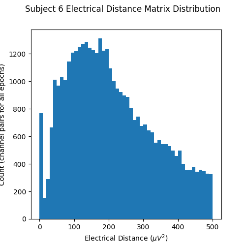
现在绘制电距离矩阵的直方图。注意上一幅图的电距离矩阵是上三角且不含对角线，因此成对电距离并非在同一通道之间计算（通道与自身的差异显然为零）。靠近零的初始峰因此代表不同通道几乎相同的配对，提示短接；没有短接电极的 EEG 记录不会在零附近出现峰。

fig, ax = plt.subplots(figsize=(5, 5))
fig.suptitle("Subject 6 Electrical Distance Matrix Distribution")
ax.hist(ed_matrix[~np.isnan(ed_matrix)], bins=np.linspace(0, 500, 51))
ax.set_xlabel(r"Electrical Distance ($\mu$$V^2$)")
ax.set_ylabel("Count (channel pairs for all epochs)")

Subject 6 Electrical Distance Matrix Distribution

在地形图上绘制电距离#

再看电距离矩阵的地形图，找出短接通道的位置并确认其空间排列是否合理。这里对每个通道取最小电距离，并在所有分段上取中位数（原始数据按 2 秒不重叠区间分段）。该示例是 EEGBCI 数据集中短接通道最多的受试者，因此有许多浅色区域与红线。它们通常成组出现，且偏向水平连接（这可能因为 EEG 实验者常站在侧面，凝胶注射器尖端插入过深）。

mne.viz.plot_bridged_electrodes(
    raw_data[6].info,
    bridged_idx,
    ed_matrix,
    title="Subject 6 Bridged Electrodes",
    topomap_args=dict(vlim=(None, 5)),
)

绘制短接电极的原始电压时间序列#

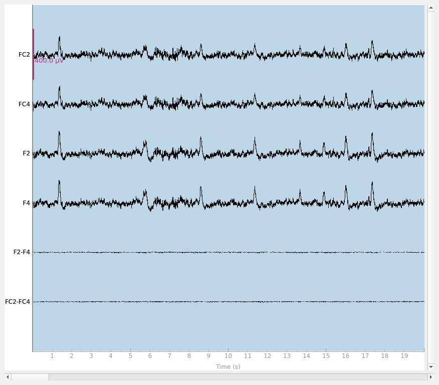
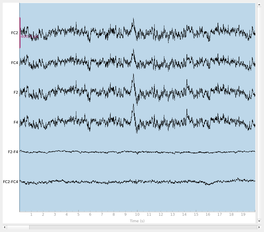
最后做基本检查，确认短接电极确实相似得不合常理。我们绘制两对短接电极 F2-F4 与 FC2-FC4，分别看受试者 6（短接）与受试者 1（未短接）。可以看到，受试者 6 的配对几乎完全相同，证实很可能短接。有趣的是，尽管两对彼此相邻，却形成两个不同的配对，说明这四个电极不太可能全部短接。

raw = raw_data[6].copy().pick(["FC2", "FC4", "F2", "F4"])
raw.add_channels(
    [
        mne.io.RawArray(
            raw.get_data(ch1) - raw.get_data(ch2),
            mne.create_info([f"{ch1}-{ch2}"], raw.info["sfreq"], "eeg"),
            raw.first_samp,
        )
        for ch1, ch2 in [("F2", "F4"), ("FC2", "FC4")]
    ]
)
raw.plot(duration=20, scalings=dict(eeg=2e-4))

raw = raw_data[1].copy().pick(["FC2", "FC4", "F2", "F4"])
raw.add_channels(
    [
        mne.io.RawArray(
            raw.get_data(ch1) - raw.get_data(ch2),
            mne.create_info([f"{ch1}-{ch2}"], raw.info["sfreq"], "eeg"),
            raw.first_samp,
        )
        for ch1, ch2 in [("F2", "F4"), ("FC2", "FC4")]
    ]
)
raw.plot(duration=20, scalings=dict(eeg=2e-4))

Creating RawArray with float64 data, n_channels=1, n_times=9760
    Range : 0 ... 9759 =      0.000 ...    60.994 secs
Ready.
Creating RawArray with float64 data, n_channels=1, n_times=9760
    Range : 0 ... 9759 =      0.000 ...    60.994 secs
Ready.
Using qt as 2D backend.
Creating RawArray with float64 data, n_channels=1, n_times=9760
    Range : 0 ... 9759 =      0.000 ...    60.994 secs
Ready.
Creating RawArray with float64 data, n_channels=1, n_times=9760
    Range : 0 ... 9759 =      0.000 ...    60.994 secs
Ready.

在 EEGBCI 数据集中比较不同受试者的短接情况#

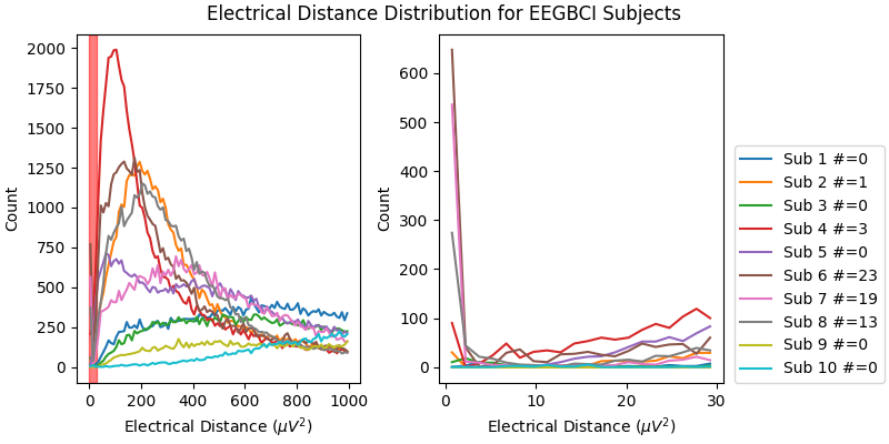
现在查看整个 EEGBCI 数据集的电距离直方图。如右侧放大插图所示，受试者 6、7、8（以及程度较轻的 2、4）在 0 \({\mu}V^2\) 附近的分布形状与其他受试者不同：这些受试者的分布在 0 \({\mu}V^2\) 附近有峰、在 5 \({\mu}V^2\) 附近有谷，提示电极短接。其余受试者的分布单调上升，说明源的空间分离正常。分布形状的巨大差异可能主要来自眨眼等伪迹（其幅度比神经数据大一个数量级，因为该数据未做预处理），但也可能反映神经或至少解剖上的差异（即传感器到大脑的距离）。

fig, (ax1, ax2) = plt.subplots(1, 2, figsize=(8, 4), layout="constrained")
fig.suptitle("Electrical Distance Distribution for EEGBCI Subjects")
for ax in (ax1, ax2):
    ax.set_ylabel("Count")
    ax.set_xlabel(r"Electrical Distance ($\mu$$V^2$)")

for sub, (bridged_idx, ed_matrix) in ed_data.items():
    # ed_matrix is upper triangular so exclude bottom half of NaNs
    hist, edges = np.histogram(
        ed_matrix[~np.isnan(ed_matrix)].flatten(), bins=np.linspace(0, 1000, 101)
    )
    centers = (edges[1:] + edges[:-1]) / 2
    ax1.plot(centers, hist)
    hist, edges = np.histogram(
        ed_matrix[~np.isnan(ed_matrix)].flatten(), bins=np.linspace(0, 30, 21)
    )
    centers = (edges[1:] + edges[:-1]) / 2
    ax2.plot(centers, hist, label=f"Sub {sub} #={len(bridged_idx)}")

ax1.axvspan(0, 30, color="r", alpha=0.5)
ax2.legend(loc=(1.04, 0))

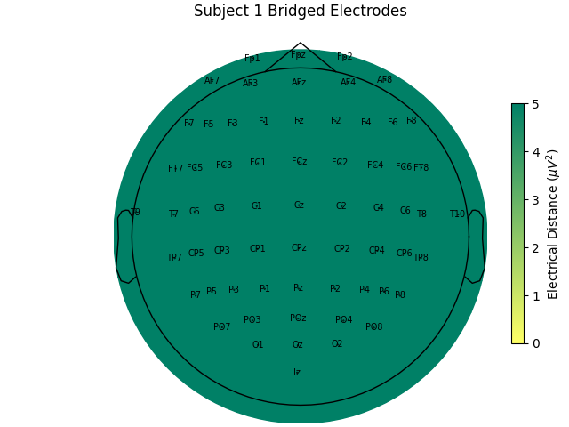
Electrical Distance Distribution for EEGBCI Subjects

对整组受试者查看其电距离与短接情况。尤其因为这是同一任务，许多受试者缺乏低电距离，有力说明低电距离由短接造成，并且只要更谨慎地施加凝胶或其他导电电解质便可避免。

for sub, (bridged_idx, ed_matrix) in ed_data.items():
    mne.viz.plot_bridged_electrodes(
        raw_data[sub].info,
        bridged_idx,
        ed_matrix,
        title=f"Subject {sub} Bridged Electrodes",
        topomap_args=dict(vlim=(None, 5)),
    )

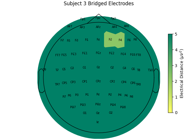
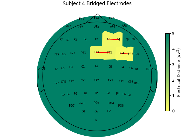
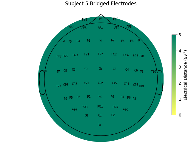
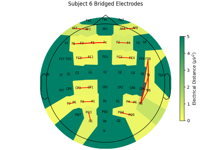
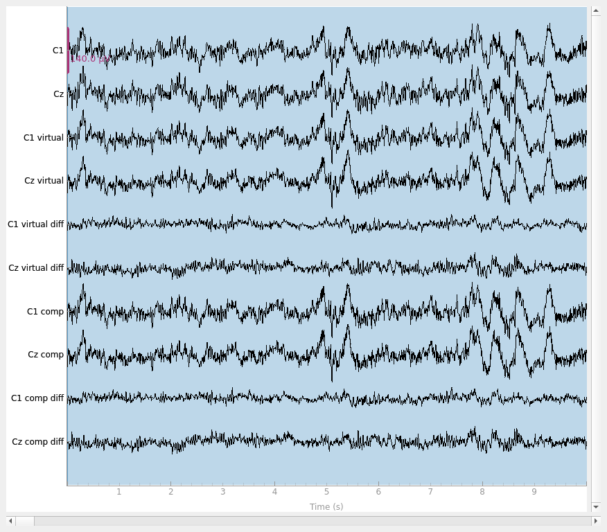
对像上例受试者 6 这样短接通道很多的受试者，建议排除该受试者，因为其 EEG 电极布局无法与其他受试者比较；若尝试插值，插值又会依赖同样短接的其他通道。而对只有少数短接通道的受试者，可对这些通道插值。由于短接数据仍是生物信号（记录的是受试者大脑），只是空间上被模糊，可用 mne.preprocessing.interpolate_bridged_electrodes() 在两个短接通道之间构造虚拟通道以辅助插值。

# use subject 2, only one bridged electrode pair
bridged_idx = ed_data[2][0]
raw = mne.preprocessing.interpolate_bridged_electrodes(
    raw_data[2].copy(), bridged_idx=bridged_idx
)

Creating RawArray with float64 data, n_channels=1, n_times=9760
    Range : 0 ... 9759 =      0.000 ...    60.994 secs
Ready.
Setting channel interpolation method to {'eeg': 'spline'}.
Interpolating bad channels.
    Automatic origin fit: head of radius 95.0 mm
Computing interpolation matrix from 63 sensor positions
Interpolating 2 sensors

我们验证虚拟通道是否有助于插值：通过模拟短接，确认虚拟通道方法能更好地恢复原始数据。把两个通道变得几乎相同以模拟短接电极，同时保存原始数据，即可比较两种插值方法。可以看到，虚拟通道略微更接近地恢复原始数据；但如图所示，两种方法都仍有残余信号，说明与未短接通道相比仍存在数据损失。

raw = raw_data[2].copy()

# pick two channels to simulate a bridge
idx0, idx1 = 9, 10
ch0, ch1 = raw.ch_names[idx0], raw.ch_names[idx1]
bridged_idx_simulated = [(idx0, idx1)]
# get the original data to compare to
data_orig = raw_data[2].get_data(picks=(idx0, idx1))

# simulate a bridge between the two channels by taking their mean and adding
# some noise
rng = np.random.default_rng(11)  # seed for reproducibility
raw_sim = raw.copy()  # raw with simulated electrode bridge
# remove channels with original data
raw_sim = raw_sim.drop_channels([ch0, ch1])
bridged_data = np.tile(np.mean(data_orig, axis=0), (2, 1))  # copy mean
# add separate noise for each channel
bridged_data[0] += 1e-7 * rng.normal(size=raw.times.size)
bridged_data[1] += 1e-7 * rng.normal(size=raw.times.size)
# add back simulated data
raw_sim = raw_sim.add_channels(
    [
        mne.io.RawArray(
            bridged_data,
            mne.create_info([ch0, ch1], raw.info["sfreq"], "eeg"),
            raw.first_samp,
        )
    ]
)
raw_sim.set_montage(montage)  # add back channel positions

# use virtual channel method
raw_virtual = mne.preprocessing.interpolate_bridged_electrodes(
    raw_sim.copy(), bridged_idx=bridged_idx_simulated
)
data_virtual = raw_virtual.get_data(picks=(idx0, idx1))

# set bads to be bridged electrodes to interpolate without a virtual channel
raw_comp = raw_sim.copy()
raw_comp.info["bads"] = [raw_sim.ch_names[idx0], raw_sim.ch_names[idx1]]
raw_comp.interpolate_bads()
data_comp = raw_comp.get_data(picks=(idx0, idx1))

# compute variance of residuals
print(
    "Variance of residual (interpolated data - original data)\n\n"
    f"With adding virtual channel:                         {np.mean(np.var(data_virtual - data_orig, axis=1))}\n"
    f"Compared to interpolation only using other channels: {np.mean(np.var(data_comp - data_orig, axis=1))}"
    ""
)

# plot results
raw = raw.pick([ch0, ch1])
raw = raw.add_channels(
    [
        mne.io.RawArray(
            np.concatenate([data_virtual, data_virtual - data_orig]),
            mne.create_info(
                [
                    f"{ch0} virtual",
                    f"{ch1} virtual",
                    f"{ch0} virtual diff",
                    f"{ch1} virtual diff",
                ],
                raw.info["sfreq"],
                "eeg",
            ),
            raw.first_samp,
        )
    ]
)
raw = raw.add_channels(
    [
        mne.io.RawArray(
            np.concatenate([data_comp, data_comp - data_orig]),
            mne.create_info(
                [f"{ch0} comp", f"{ch1} comp", f"{ch0} comp diff", f"{ch1} comp diff"],
                raw.info["sfreq"],
                "eeg",
            ),
            raw.first_samp,
        )
    ]
)
raw.plot(scalings=dict(eeg=7e-5))

Creating RawArray with float64 data, n_channels=2, n_times=9760
    Range : 0 ... 9759 =      0.000 ...    60.994 secs
Ready.
Creating RawArray with float64 data, n_channels=1, n_times=9760
    Range : 0 ... 9759 =      0.000 ...    60.994 secs
Ready.
Setting channel interpolation method to {'eeg': 'spline'}.
Interpolating bad channels.
    Automatic origin fit: head of radius 95.0 mm
Computing interpolation matrix from 63 sensor positions
Interpolating 2 sensors
Setting channel interpolation method to {'eeg': 'spline'}.
Interpolating bad channels.
    Automatic origin fit: head of radius 95.0 mm
Computing interpolation matrix from 62 sensor positions
Interpolating 2 sensors
Variance of residual (interpolated data - original data)

With adding virtual channel:                         2.055985023620412e-10
Compared to interpolation only using other channels: 2.0424942431539205e-10
Creating RawArray with float64 data, n_channels=4, n_times=9760
    Range : 0 ... 9759 =      0.000 ...    60.994 secs
Ready.
Creating RawArray with float64 data, n_channels=4, n_times=9760
    Range : 0 ... 9759 =      0.000 ...    60.994 secs
Ready.

短接与阻抗的关系#

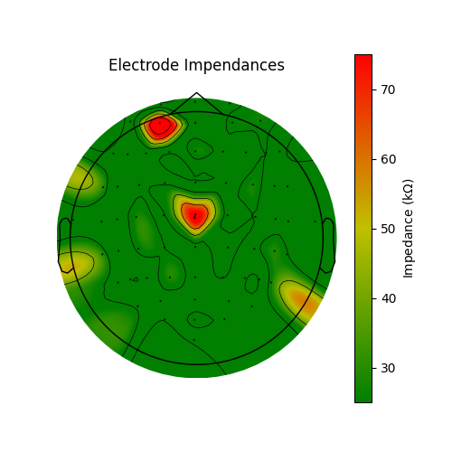
电极短接常因注入更多凝胶以降低阻抗而发生。因此，在成为理想 EEG 技术员的路上，比较短接与阻抗会很有帮助！低阻抗带来噪声更少的数据，而无短接的 EEG 空间精度更高。脑成像数据结构（BIDS）建议把阻抗存放在 EEG 数据集的 electrodes.tsv 文件中。该数据集未保存阻抗，因此我们伪造数据以演示绘制方式。这里按准备结束时常见的做法绘制阻抗：多数通道良好，少数需要降低阻抗。使用有源系统时，实验开始前阻抗最好全部低于 25 kΩ；使用无源系统时应低于 5 kΩ。

rng = np.random.default_rng(11)  # seed for reproducibility
raw = raw_data[1]
# typically impedances < 25 kOhm are acceptable for active systems and
# impedances < 5 kOhm are desirable for a passive system
impedances = rng.random(len(raw.ch_names)) * 30
impedances[10] = 80  # set a few bad impendances
impedances[25] = 99
cmap = LinearSegmentedColormap.from_list(
    name="impedance_cmap", colors=["g", "y", "r"], N=256
)
fig, ax = plt.subplots(figsize=(5, 5))
im, cn = mne.viz.plot_topomap(impedances, raw.info, axes=ax, cmap=cmap, vlim=(25, 75))
ax.set_title("Electrode Impendances")
cax = fig.colorbar(im, ax=ax)
cax.set_label(r"Impedance (k$\Omega$)")

小结#

本示例展示了一个在多名受试者的 EEG 准备过程中出现电短接的数据集。希望这能说明规范操作的重要性，以及检查自己的工作以不断学习改进的意义；也希望该工具能帮助大家今后采集更好的 EEG 数据。

参考文献#

脚本总运行时间：（0 分 6.705 秒）

图库由 Sphinx-Gallery 生成