
注意
转到末尾下载完整示例代码。
单试次功率的非参数单样本聚类统计#
本脚本展示如何估计时频功率估计中的显著聚类。它采用基于置换和聚类水平统计量的非参数统计流程。
该流程包括:
提取 Epochs
计算单试次功率估计
对功率估计进行基线校正(功率比值)
计算统计量,检验比值是否偏离 1。
这里的观测单位是来自某一特定研究被试的 Epochs。不过,当观测单位是若干研究被试、且每位被试提供自己的平均数据(即其 Epochs 的平均值)时,同样的逻辑同样适用;这种情况下的分析被视为“第二层”(2nd level)分析。
有关 MNE-Python 中基于聚类的置换检验的更多信息,另请参阅:全传感器数据的时空置换 F 检验(全传感器数据的时空置换 F 检验)。
# Authors: Alexandre Gramfort <alexandre.gramfort@inria.fr>
#          Stefan Appelhoff <stefan.appelhoff@mailbox.org>
#
# License: BSD-3-Clause
# Copyright the MNE-Python contributors.
import matplotlib.pyplot as plt
import numpy as np
import scipy.stats

import mne
from mne.datasets import sample
from mne.stats import permutation_cluster_1samp_test
设置参数#
data_path = sample.data_path()
meg_path = data_path / "MEG" / "sample"
raw_fname = meg_path / "sample_audvis_raw.fif"
tmin, tmax, event_id = -0.3, 0.6, 1

# Setup for reading the raw data
raw = mne.io.read_raw_fif(raw_fname)
events = mne.find_events(raw, stim_channel="STI 014")

include = []
raw.info["bads"] += ["MEG 2443", "EEG 053"]  # bads + 2 more

# for speed, we'll only look at right-temporal gradiometers (and EOG)
picks_eog = mne.pick_types(raw.info, eog=True)
picks_grad = mne.pick_types(raw.info, meg="grad", exclude="bads")
picks_rtemp = mne.pick_channels(
    raw.info["ch_names"], mne.read_vectorview_selection("Right-temporal"), ordered=True
)
picks = list((set(picks_rtemp) & set(picks_grad)) | set(picks_eog))

# Load condition 1
event_id = 1
epochs = mne.Epochs(
    raw,
    events,
    event_id,
    tmin,
    tmax,
    picks=picks,
    baseline=(None, 0),
    preload=True,
    reject=dict(grad=4000e-13, eog=150e-6),
)

evoked = epochs.average()

# Factor to down-sample the temporal dimension of the TFR computed by
# tfr_morlet. Decimation occurs after frequency decomposition and can
# be used to reduce memory usage (and possibly computational time of downstream
# operations such as nonparametric statistics) if you don't need high
# spectrotemporal resolution.
decim = 5

# define frequencies of interest
freqs = np.arange(8, 40, 2)

# run the TFR decomposition
tfr_epochs = epochs.compute_tfr(
    "morlet",
    freqs,
    n_cycles=4.0,
    decim=decim,
    average=False,
    return_itc=False,
    n_jobs=None,
)

# Baseline power
tfr_epochs.apply_baseline(mode="logratio", baseline=(-0.100, 0))

# Crop in time to keep only what is between 0 and 400 ms
evoked.crop(-0.1, 0.4)
tfr_epochs.crop(-0.1, 0.4)

epochs_power = tfr_epochs.data
Opening raw data file /home/circleci/mne_data/MNE-sample-data/MEG/sample/sample_audvis_raw.fif...
    Read a total of 3 projection items:
        PCA-v1 (1 x 10²)  idle
        PCA-v2 (1 x 10²)  idle
        PCA-v3 (1 x 10²)  idle
    Range : 25800 ... 192599 =     42.956 ...   320.670 secs
Ready.
Finding events on: STI 014
320 events found on stim channel STI 014
Event IDs: [ 1  2  3  4  5 32]
Not setting metadata
72 matching events found
Setting baseline interval to [-0.2996928197375818, 0.0] s
Applying baseline correction (mode: mean)
0 projection items activated
Loading data for 72 events and 541 original time points ...
    Rejecting  epoch based on EOG : ['EOG 061']
    Rejecting  epoch based on EOG : ['EOG 061']
    Rejecting  epoch based on EOG : ['EOG 061']
    Rejecting  epoch based on EOG : ['EOG 061']
    Rejecting  epoch based on EOG : ['EOG 061']
    Rejecting  epoch based on EOG : ['EOG 061']
    Rejecting  epoch based on EOG : ['EOG 061']
    Rejecting  epoch based on EOG : ['EOG 061']
    Rejecting  epoch based on EOG : ['EOG 061']
    Rejecting  epoch based on EOG : ['EOG 061']
    Rejecting  epoch based on EOG : ['EOG 061']
    Rejecting  epoch based on EOG : ['EOG 061']
    Rejecting  epoch based on EOG : ['EOG 061']
    Rejecting  epoch based on EOG : ['EOG 061']
    Rejecting  epoch based on EOG : ['EOG 061']
    Rejecting  epoch based on EOG : ['EOG 061']
    Rejecting  epoch based on EOG : ['EOG 061']
    Rejecting  epoch based on EOG : ['EOG 061']
18 bad epochs dropped
Applying baseline correction (mode: logratio)
定义统计所需的邻接关系#
要执行基于聚类的置换检验,我们需要为传感器、时间点和频率点的邻接关系给出合适的定义。邻接矩阵将用于形成聚类。
我们首先计算传感器邻接关系,然后将其与时频平面的“格点”邻接关系相结合。后者假定索引为“N”的元素与索引为“N + 1”和“N - 1”的元素相邻(从而在时频平面上形成一个“网格”)。
# find_ch_adjacency first attempts to find an existing "neighbor"
# (adjacency) file for given sensor layout.
# If such a file doesn't exist, an adjacency matrix is computed on the fly,
# using Delaunay triangulations.
sensor_adjacency, ch_names = mne.channels.find_ch_adjacency(tfr_epochs.info, "grad")

# In this case, find_ch_adjacency finds an appropriate file and
# reads it (see log output: "neuromag306planar").
# However, we need to subselect the channels we are actually using
use_idx = [ch_names.index(ch_name) for ch_name in tfr_epochs.ch_names]
sensor_adjacency = sensor_adjacency[use_idx][:, use_idx]

# Our sensor adjacency matrix is of shape n_chs × n_chs
assert sensor_adjacency.shape == (len(tfr_epochs.ch_names), len(tfr_epochs.ch_names))

# Now we need to prepare adjacency information for the time-frequency
# plane. For that, we use "combine_adjacency", and pass dimensions
# as in the data we want to test (excluding observations). Here:
# channels × frequencies × times
assert epochs_power.data.shape == (
    len(epochs),
    len(tfr_epochs.ch_names),
    len(tfr_epochs.freqs),
    len(tfr_epochs.times),
)
adjacency = mne.stats.combine_adjacency(
    sensor_adjacency, len(tfr_epochs.freqs), len(tfr_epochs.times)
)

# The overall adjacency we end up with is a square matrix with each
# dimension matching the data size (excluding observations) in an
# "unrolled" format, so: len(channels × frequencies × times)
assert (
    adjacency.shape[0]
    == adjacency.shape[1]
    == len(tfr_epochs.ch_names) * len(tfr_epochs.freqs) * len(tfr_epochs.times)
)
Reading adjacency matrix for neuromag306planar.
计算统计量#
为形成聚类,我们需要指定一个临界检验统计量阈值。只有超过该阈值的数据点才会被用于形成聚类。
这里我们使用 t 检验,并可以利用 SciPy 中 t 分布的百分点函数(percent point function)获得对应于特定显著性 alpha 水平的 t 值。该阈值通常称为“聚类形成阈值”(cluster forming threshold)。
注意
阈值的选择多少有些任意。选择对应于 p=0.05、p=0.01 或 p=0.001 的 t 值通常是一个不错的起点。具体取决于你所分析的数据集,你可能需要调整该阈值。
# We want a two-tailed test
tail = 0

# In this example, we wish to set the threshold for including data bins in
# the cluster forming process to the t-value corresponding to p=0.001 for the
# given data.
#
# Because we conduct a two-tailed test, we divide the p-value by 2 (which means
# we're making use of both tails of the distribution).
# As the degrees of freedom, we specify the number of observations
# (here: epochs) minus 1.
# Finally, we subtract 0.001 / 2 from 1, to get the critical t-value
# on the right tail (this is needed for MNE-Python internals)
degrees_of_freedom = len(epochs) - 1
t_thresh = scipy.stats.t.ppf(1 - 0.001 / 2, df=degrees_of_freedom)

# Set the number of permutations to run.
# Warning: 50 is way too small for a real-world analysis (where values of 5000
# or higher are used), but here we use it to increase the computation speed.
n_permutations = 50

# Run the analysis
T_obs, clusters, cluster_p_values, H0 = permutation_cluster_1samp_test(
    epochs_power,
    n_permutations=n_permutations,
    threshold=t_thresh,
    tail=tail,
    adjacency=adjacency,
    out_type="mask",
    rng=73,
    verbose=True,
)
stat_fun(H1): min=-6.455144461077351 max=8.265125482991843
Running initial clustering …
Found 47 clusters

  0%|          | Permuting : 0/49 [00:00<?,       ?it/s]
 61%|██████    | Permuting : 30/49 [00:00<00:00,  830.05it/s]
100%|██████████| Permuting : 49/49 [00:00<00:00,  862.87it/s]
100%|██████████| Permuting : 49/49 [00:00<00:00,  859.00it/s]
查看时频图#
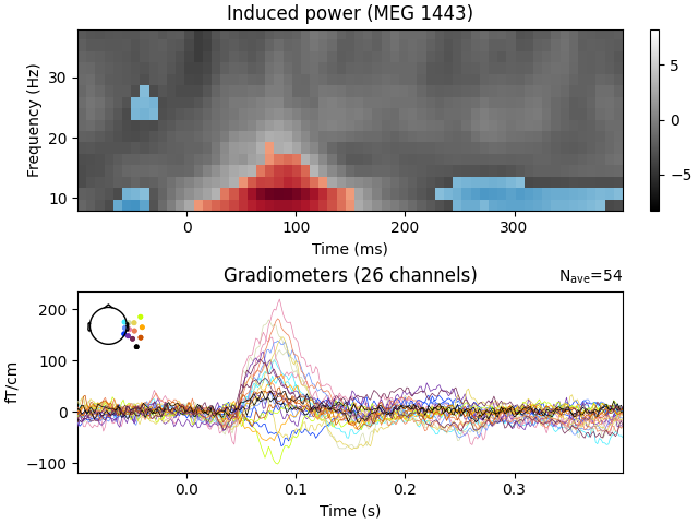
现在我们将可视化在置换分布下具有统计显著性的观测聚类。
警告
谈论“显著聚类”可能很方便,但你必须意识到所有相关的注意事项!例如,将聚类 p 值解释为具有空间或时间特异性是无效的。某个特定位置上 p 值足够低(例如 < 0.05)的聚类,并不能让你断言显著效应就位于该特定位置。p 值只告诉你:在比较的条件之间没有差异的情况下,在数据的任意位置获得相似或更强/更大聚类的概率。因此,它只允许你对数据“总体上”的差异得出结论,而不能针对特定位置。更多信息请参阅详尽的 FieldTrip 教程。更多信息请参阅 FieldTrip 教程。
evoked_data = evoked.data
times = 1e3 * evoked.times

fig, (ax, ax2) = plt.subplots(2, layout="constrained")

T_obs_plot = np.nan * np.ones_like(T_obs)
for c, p_val in zip(clusters, cluster_p_values):
    if p_val <= 0.05:
        T_obs_plot[c] = T_obs[c]

# Just plot one channel's data
# use the following to show a specific one:
# ch_idx = tfr_epochs.ch_names.index('MEG 1332')
ch_idx, f_idx, t_idx = np.unravel_index(
    np.nanargmax(np.abs(T_obs_plot)), epochs_power.shape[1:]
)

vmax = np.max(np.abs(T_obs))
vmin = -vmax
ax.imshow(
    T_obs[ch_idx],
    cmap=plt.cm.gray,
    extent=[times[0], times[-1], freqs[0], freqs[-1]],
    aspect="auto",
    origin="lower",
    vmin=vmin,
    vmax=vmax,
)
ax.imshow(
    T_obs_plot[ch_idx],
    cmap=plt.cm.RdBu_r,
    extent=[times[0], times[-1], freqs[0], freqs[-1]],
    aspect="auto",
    origin="lower",
    vmin=vmin,
    vmax=vmax,
)
fig.colorbar(ax.images[0])
ax.set(xlabel="Time (ms)", ylabel="Frequency (Hz)")
ax.set(title=f"Induced power ({tfr_epochs.ch_names[ch_idx]})")

evoked.plot(axes=[ax2], time_unit="s")
脚本总运行时间:(0 分钟 1.022 秒)