使用时空谱分解（SSD）计算空间滤波器#

本示例按 [1] 的建议计算空间滤波器，以保留振荡性脑活动并降低 1/f 背景信号的权重。其思路是基于感兴趣频段的协方差与周围频率的噪声协方差，学习能把振荡动态与周围非振荡噪声分离的空间滤波器。

# Author: Denis A. Engemann <denis.engemann@gmail.com>
#         Victoria Peterson <victoriapeterson09@gmail.com>
# License: BSD-3-Clause
# Copyright the MNE-Python contributors.

import matplotlib.pyplot as plt

import mne
from mne import Epochs
from mne.datasets.fieldtrip_cmc import data_path
from mne.decoding import SSD, get_spatial_filter_from_estimator

定义参数

fname = data_path() / "SubjectCMC.ds"

# Prepare data
raw = mne.io.read_raw_ctf(fname)
raw.crop(tmin=50.0, tmax=110.0).load_data()  # crop for memory purposes
raw.resample(sfreq=250)

raw.pick_types(meg=True, ref_meg=False)

freqs_sig = 9, 12
freqs_noise = 8, 13


ssd = SSD(
    info=raw.info,
    reg="oas",
    sort_by_spectral_ratio=False,  # False for purpose of example.
    filt_params_signal=dict(
        l_freq=freqs_sig[0],
        h_freq=freqs_sig[1],
        l_trans_bandwidth=1,
        h_trans_bandwidth=1,
    ),
    filt_params_noise=dict(
        l_freq=freqs_noise[0],
        h_freq=freqs_noise[1],
        l_trans_bandwidth=1,
        h_trans_bandwidth=1,
    ),
)
ssd.fit(X=raw.get_data())

ds directory : /home/circleci/mne_data/MNE-fieldtrip_cmc-data/SubjectCMC.ds
    res4 data read.
    hc data read.
    Separate EEG position data file not present.
    Quaternion matching (desired vs. transformed):
       0.33   78.32    0.00 mm <->    0.33   78.32    0.00 mm (orig :  -71.62   40.46 -256.48 mm) diff =    0.000 mm
      -0.33  -78.32   -0.00 mm <->   -0.33  -78.32   -0.00 mm (orig :   39.27  -70.16 -258.60 mm) diff =    0.000 mm
     114.65    0.00   -0.00 mm <->  114.65    0.00   -0.00 mm (orig :   64.35   66.64 -262.01 mm) diff =    0.000 mm
    Coordinate transformations established.
    Polhemus data for 3 HPI coils added
    Device coordinate locations for 3 HPI coils added
Picked positions of 4 EEG channels from channel info
    4 EEG locations added to Polhemus data.
    Measurement info composed.
Finding samples for /home/circleci/mne_data/MNE-fieldtrip_cmc-data/SubjectCMC.ds/SubjectCMC.meg4:
    System clock channel is available, checking which samples are valid.
    75 x 12000 = 911610 samples from 191 chs
    390 samples omitted at the end
Current compensation grade : 0
Reading 0 ... 72000  =      0.000 ...    60.000 secs...
Finding events on: STIM
29 events found on stim channel STIM
Event IDs: [   196608    262144    327680    393216    458752  67108864  67174400
 134742016 136314880 268435456]
Finding events on: STIM
29 events found on stim channel STIM
Event IDs: [   196608    262144    327680    393216    458752  67108864  67174400
 134742016 136314880 268435456]
NOTE: pick_types() is a legacy function. New code should use inst.pick(...).
Removing 5 compensators from info because not all compensation channels were picked.
Setting up band-pass filter from 9 - 12 Hz

FIR filter parameters
---------------------
Designing a one-pass, zero-phase, non-causal bandpass filter:
- Windowed time-domain design (firwin) method
- Hamming window with 0.0194 passband ripple and 53 dB stopband attenuation
- Lower passband edge: 9.00
- Lower transition bandwidth: 1.00 Hz (-6 dB cutoff frequency: 8.50 Hz)
- Upper passband edge: 12.00 Hz
- Upper transition bandwidth: 1.00 Hz (-6 dB cutoff frequency: 12.50 Hz)
- Filter length: 825 samples (3.300 s)

Setting up band-pass filter from 8 - 13 Hz

FIR filter parameters
---------------------
Designing a one-pass, zero-phase, non-causal bandpass filter:
- Windowed time-domain design (firwin) method
- Hamming window with 0.0194 passband ripple and 53 dB stopband attenuation
- Lower passband edge: 8.00
- Lower transition bandwidth: 1.00 Hz (-6 dB cutoff frequency: 7.50 Hz)
- Upper passband edge: 13.00 Hz
- Upper transition bandwidth: 1.00 Hz (-6 dB cutoff frequency: 13.50 Hz)
- Filter length: 825 samples (3.300 s)

Estimating covariance using OAS
Done.
Estimating covariance using OAS
Done.
Computing rank from covariance with rank=None
    Using tolerance 1.2e-14 (2.2e-16 eps * 151 dim * 0.37  max singular value)
    Estimated rank (mag): 151
    MAG: rank 151 computed from 151 data channels with 0 projectors
Computing rank from covariance with rank=None
    Using tolerance 2.9e-15 (2.2e-16 eps * 151 dim * 0.086  max singular value)
    Estimated rank (mag): 151
    MAG: rank 151 computed from 151 data channels with 0 projectors
Done.

SSD(filt_params_noise={'h_freq': 13, 'h_trans_bandwidth': 1, 'l_freq': 8,
                       'l_trans_bandwidth': 1},
    filt_params_signal={'h_freq': 12, 'h_trans_bandwidth': 1, 'l_freq': 9,
                        'l_trans_bandwidth': 1},
    info=<Info | 14 non-empty values
 bads: []
 ch_names: MLC11-1706, MLC12-1706, MLC13-1706, MLC14-1706, MLC15-1706, ...
 chs: 151 Magnetometers
 ctf_head_t: CTF/4D/KIT head -> head transform
 custom_re...ed: False
 dev_ctf_t: MEG device -> CTF/4D/KIT head transform
 dev_head_t: MEG device -> head transform
 dig: 7 items (3 Cardinal, 4 EEG)
 highpass: 0.0 Hz
 hpi_results: 1 item (list)
 lowpass: 125.0 Hz
 meas_date: 2005-01-31 14:43:00 UTC
 meas_id: 4 items (dict)
 nchan: 151
 projs: []
 sfreq: 250.0 Hz
 subject_info: <subject_info | his_id: Anonymized25263_1299153182_0>
>,
    reg='oas', sort_by_spectral_ratio=False)

In a Jupyter environment, please rerun this cell to show the HTML representation or trust the notebook.
On GitHub, the HTML representation is unable to render, please try loading this page with nbviewer.org.

SSD

iFitted

Parameters

	info	<Info \| 14 no...299153182_0> >
	filt_params_signal	{'h_freq': 12, 'h_trans_bandwidth': 1, 'l_freq': 9, 'l_trans_bandwidth': 1}
	filt_params_noise	{'h_freq': 13, 'h_trans_bandwidth': 1, 'l_freq': 8, 'l_trans_bandwidth': 1}
	reg	'oas'
	sort_by_spectral_ratio	False
	n_components	None
	picks	None
	return_filtered	False
	n_fft	None
	cov_method_params	None
	restr_type	'whitening'
	rank	None

Fitted attributes

Name	Type	Value
evals_	ndarray[float64](151,)	[35.9 ,34.46,26.97,..., 0.49, 0.48, 0.41]
filters_	ndarray[float64](151, 151)	[[ 8.31e+12,-2.07e+13,-3.72e+13,...,-3.11e+13,-3.67e+13, 1.37e+13], [-4.90e+12,-3.48e+12,-4.51e+13,...,-2.97e+13, 8.18e+11,-2.28e+13], [ 1.41e+13,-1.98e+13,-8.97e+12,..., 1.54e+13, 3.17e+13,-7.70e+12], ..., [-7.59e+12,-1.96e+13, 6.89e+12,..., 7.53e+12, 7.78e+12, 9.72e+12], [-8.19e+12,-2.27e+13, 1.72e+12,..., 1.64e+12, 7.32e+12, 2.65e+12], [ 1.19e+13, 9.69e+12,-6.84e+12,..., 3.31e+12, 1.29e+13, 4.21e+12]]
freqs_noise_	tuple	(8, 13)
freqs_signal_	tuple	(9, 12)
n_features_in_	int	15000
n_fft_	int	250
patterns_	ndarray[float64](151, 151)	[[ 0., 0., 0.,..., 0., 0., 0.], [ 0., 0., 0.,...,-0., 0., 0.], [ 0., 0., 0.,...,-0., 0., 0.], ..., [-0.,-0., 0.,...,-0.,-0.,-0.], [ 0., 0., 0.,...,-0.,-0.,-0.], [ 0.,-0.,-0.,..., 0.,-0.,-0.]]
picks_	ndarray[int64](151,)	[ 0, 1, 2,...,148,149,150]
sfreq_	float	250
sorter_	ndarray[int64](151,)	[150,149,148,..., 2, 1, 0]

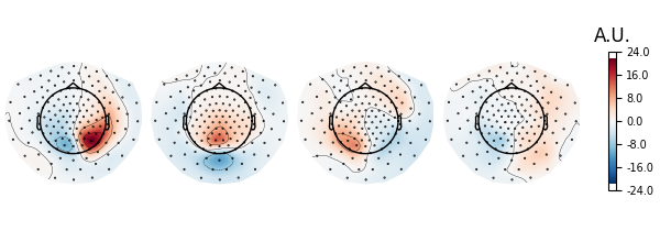
我们先考察功率比最大的空间滤波器，查看其地形图。根据 Nikulin 等人（2011）的做法，可以通过反转滤波器（W^{-1}）或把噪声协方差与滤波器相乘 Eq. (22)（C_n W)^t 得到。这里采用反转方法。

spf = get_spatial_filter_from_estimator(ssd, info=ssd.info)
spf.plot_patterns(components=list(range(4)))

# The topographies suggest that we picked up a parietal alpha generator.

# Transform
ssd_sources = ssd.transform(X=raw.get_data())

# Get psd of SSD-filtered signals.
psd, freqs = mne.time_frequency.psd_array_welch(
    ssd_sources, sfreq=raw.info["sfreq"], n_fft=4096
)

# Get spec_ratio information (already sorted)
# Note that this is not necessary if sort_by_spectral_ratio=True (default)
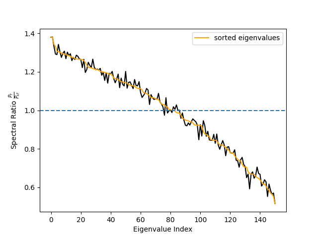
spec_ratio, sorter = ssd.get_spectral_ratio(ssd_sources)

# Plot spectral ratio (see Eq. 24 in Nikulin et al., 2011).
fig, ax = plt.subplots(1)
ax.plot(spec_ratio, color="black")
ax.plot(spec_ratio[sorter], color="orange", label="sorted eigenvalues")
ax.set_xlabel("Eigenvalue Index")
ax.set_ylabel(r"Spectral Ratio $\frac{P_f}{P_{sf}}$")
ax.legend()
ax.axhline(1, linestyle="--")

# We can see that the initial sorting based on the eigenvalues
# was already quite good. However, when using few components only
# the sorting might make a difference.

Effective window size : 16.384 (s)
Effective window size : 1.000 (s)

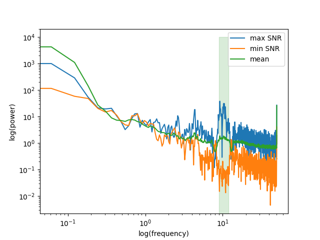
再看该源的功率谱，并与信噪比最低的源的功率谱比较。

below50 = freqs < 50
# for highlighting the freq. band of interest
bandfilt = (freqs_sig[0] <= freqs) & (freqs <= freqs_sig[1])
fig, ax = plt.subplots(1)
ax.loglog(freqs[below50], psd[0, below50], label="max SNR")
ax.loglog(freqs[below50], psd[-1, below50], label="min SNR")
ax.loglog(freqs[below50], psd[:, below50].mean(axis=0), label="mean")
ax.fill_between(freqs[bandfilt], 0, 10000, color="green", alpha=0.15)
ax.set_xlabel("log(frequency)")
ax.set_ylabel("log(power)")
ax.legend()

# We can clearly see that the selected component enjoys an SNR that is
# way above the average power spectrum.

分段数据#

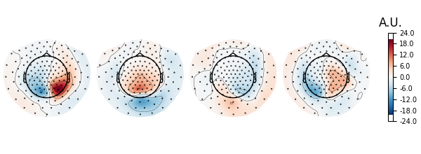
虽然我们建议在分段之前使用该方法，但有些情况下数据只能按块处理。

# Build epochs as sliding windows over the continuous raw file.
events = mne.make_fixed_length_events(raw, id=1, duration=5.0, overlap=0.0)

# Epoch length is 5 seconds.
epochs = Epochs(raw, events, tmin=0.0, tmax=5, baseline=None, preload=True)

ssd_epochs = SSD(
    info=epochs.info,
    reg="oas",
    filt_params_signal=dict(
        l_freq=freqs_sig[0],
        h_freq=freqs_sig[1],
        l_trans_bandwidth=1,
        h_trans_bandwidth=1,
    ),
    filt_params_noise=dict(
        l_freq=freqs_noise[0],
        h_freq=freqs_noise[1],
        l_trans_bandwidth=1,
        h_trans_bandwidth=1,
    ),
)
ssd_epochs.fit(X=epochs.get_data(copy=False))

# Plot topographies.
spf = get_spatial_filter_from_estimator(ssd_epochs, info=ssd_epochs.info)
spf.plot_patterns(components=list(range(4)))

Pattern0, Pattern1, Pattern2, Pattern3, AU

Not setting metadata
12 matching events found
No baseline correction applied
0 projection items activated
Using data from preloaded Raw for 12 events and 1251 original time points ...
1 bad epochs dropped
Setting up band-pass filter from 9 - 12 Hz

FIR filter parameters
---------------------
Designing a one-pass, zero-phase, non-causal bandpass filter:
- Windowed time-domain design (firwin) method
- Hamming window with 0.0194 passband ripple and 53 dB stopband attenuation
- Lower passband edge: 9.00
- Lower transition bandwidth: 1.00 Hz (-6 dB cutoff frequency: 8.50 Hz)
- Upper passband edge: 12.00 Hz
- Upper transition bandwidth: 1.00 Hz (-6 dB cutoff frequency: 12.50 Hz)
- Filter length: 825 samples (3.300 s)

Setting up band-pass filter from 8 - 13 Hz

FIR filter parameters
---------------------
Designing a one-pass, zero-phase, non-causal bandpass filter:
- Windowed time-domain design (firwin) method
- Hamming window with 0.0194 passband ripple and 53 dB stopband attenuation
- Lower passband edge: 8.00
- Lower transition bandwidth: 1.00 Hz (-6 dB cutoff frequency: 7.50 Hz)
- Upper passband edge: 13.00 Hz
- Upper transition bandwidth: 1.00 Hz (-6 dB cutoff frequency: 13.50 Hz)
- Filter length: 825 samples (3.300 s)

Estimating covariance using OAS
Done.
Estimating covariance using OAS
Done.
Computing rank from covariance with rank=None
    Using tolerance 1.3e-14 (2.2e-16 eps * 151 dim * 0.38  max singular value)
    Estimated rank (mag): 151
    MAG: rank 151 computed from 151 data channels with 0 projectors
Computing rank from covariance with rank=None
    Using tolerance 3e-15 (2.2e-16 eps * 151 dim * 0.09  max singular value)
    Estimated rank (mag): 151
    MAG: rank 151 computed from 151 data channels with 0 projectors
Effective window size : 1.000 (s)
Done.

参考文献#

脚本总运行时间：（0 分 2.123 秒）

图库由 Sphinx-Gallery 生成