非官方中文翻译本页译自 MNE-Python 官方文档：查看英文原文 ↗。文档版权归 MNE Developers 所有（BSD-3-Clause）。

注意

转到末尾下载完整示例代码。

统计推断#

本节将以入门方式简要介绍推断统计中的多个概念，并演示如何使用 MNE 的一些统计函数。

# Authors: Eric Larson <larson.eric.d@gmail.com>
#
# License: BSD-3-Clause
# Copyright the MNE-Python contributors.

from functools import partial

import matplotlib.pyplot as plt
import numpy as np
from mpl_toolkits.mplot3d import Axes3D  # noqa: F401, analysis:ignore
from scipy import stats

import mne
from mne.stats import (
    bonferroni_correction,
    fdr_correction,
    permutation_cluster_1samp_test,
    permutation_t_test,
    ttest_1samp_no_p,
)

假设检验#

零假设#

摘自维基百科：

在推断统计中，指一种一般性陈述或默认立场，即两个被测量的现象之间不存在关系，或各组之间不存在关联。

我们通常希望以一定的概率拒绝零假设（例如 p < 0.05）。这一概率也称为显著性水平 $\alpha$。为了理解其含义，我们沿用 [1] 中的示例，构造一个玩具数据集：一个 40 × 40 的方阵，中心存在“信号”，并加入白噪声、施加高斯平滑核。

width = 40
n_subjects = 10
signal_mean = 100
signal_sd = 100
noise_sd = 0.01
gaussian_sd = 5
sigma = 1e-3  # sigma for the "hat" method
n_permutations = "all"  # run an exact test
n_src = width * width

# For each "subject", make a smoothed noisy signal with a centered peak
rng = np.random.default_rng(2)
X = rng.normal(scale=noise_sd, size=(n_subjects, width, width))
# Add a signal at the center
X[:, width // 2, width // 2] = rng.normal(
    loc=signal_mean, scale=signal_sd, size=n_subjects
)
# Spatially smooth with a 2D Gaussian kernel
size = width // 2 - 1
gaussian = np.exp(-(np.arange(-size, size + 1) ** 2 / float(gaussian_sd**2)))
for si in range(X.shape[0]):
    for ri in range(X.shape[1]):
        X[si, ri, :] = np.convolve(X[si, ri, :], gaussian, "same")
    for ci in range(X.shape[2]):
        X[si, :, ci] = np.convolve(X[si, :, ci], gaussian, "same")

对所有受试者平均后的数据如下所示：

fig, ax = plt.subplots(layout="constrained")
ax.imshow(X.mean(0), cmap="inferno")
ax.set(xticks=[], yticks=[], title="Data averaged over subjects")

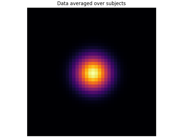
在这种情况下，我们可以针对每个体素检验的零假设是：

均值与零之间没有差异（$H_0 \colon \mu = 0$）。

相应地，备择假设是该体素的均值不为零（$H_1 \colon \mu \neq 0$）。这是双尾检验，因为均值可能小于或大于零；而单尾检验只检验其中一种可能，即 $H_1 \colon \mu \geq 0$ 或 $H_1 \colon \mu \leq 0$。

注意

这里我们将每个空间位置称为一个“体素”。不过一般而言，它可以是任何类型的数据值，包括特定时刻的皮层顶点、时频分解中的像素等。

参数检验#

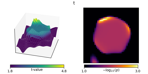
我们先从配对 t 检验（paired t-test）开始，它是检验配对样本差异的标准方法。在数学上，它等价于对每种条件下样本之间的差值做单样本 t 检验。配对 t 检验是参数检验，因为它假定潜在的样本分布为高斯分布，且仅在这种情况下有效。我们的玩具数据恰好满足这一条件，但神经影像数据并不总是满足。

在我们的玩具数据集中，体素数量很多（$40 \cdot 40 = 1600$），对每个体素分别应用配对 t 检验被称为 mass-univariate（质量单变量）方法，因为它独立地处理每个体素。

titles = ["t"]
out = stats.ttest_1samp(X, 0, axis=0)
ts = [out[0]]
ps = [out[1]]
mccs = [假]  # these are not multiple-comparisons corrected


def plot_t_p(t, p, title, mcc, axes=None):
    if axes is None:
        fig = plt.figure(figsize=(6, 3), layout="constrained")
        axes = [fig.add_subplot(121, projection="3d"), fig.add_subplot(122)]
        show = 真
    else:
        show = 假

    # calculate critical t-value thresholds (2-tailed)
    p_lims = np.array([0.1, 0.001])
    df = n_subjects - 1  # degrees of freedom
    t_lims = stats.distributions.t.ppf(1 - p_lims / 2, df=df)
    p_lims = [-np.log10(p) for p in p_lims]

    # t plot
    x, y = np.mgrid[0:width, 0:width]
    surf = axes[0].plot_surface(
        x,
        y,
        np.reshape(t, (width, width)),
        rstride=1,
        cstride=1,
        linewidth=0,
        vmin=t_lims[0],
        vmax=t_lims[1],
        cmap="viridis",
    )
    axes[0].set(
        xticks=[], yticks=[], zticks=[], xlim=[0, width - 1], ylim=[0, width - 1]
    )
    axes[0].view_init(30, 15)
    cbar = axes[0].figure.colorbar(
        ax=axes[0],
        shrink=0.75,
        orientation="horizontal",
        fraction=0.1,
        pad=0.025,
        mappable=surf,
    )
    cbar.set_ticks(t_lims)
    cbar.set_ticklabels([f"{t_lim:0.1f}" for t_lim in t_lims])
    cbar.set_label("t-value")
    cbar.ax.get_xaxis().set_label_coords(0.5, -0.3)
    if not show:
        axes[0].set(title=title)
        if mcc:
            axes[0].title.set_weight("bold")
    # p plot
    use_p = -np.log10(np.reshape(np.maximum(p, 1e-5), (width, width)))
    img = axes[1].imshow(
        use_p, cmap="inferno", vmin=p_lims[0], vmax=p_lims[1], interpolation="nearest"
    )
    axes[1].set(xticks=[], yticks=[])
    cbar = axes[1].figure.colorbar(
        ax=axes[1],
        shrink=0.75,
        orientation="horizontal",
        fraction=0.1,
        pad=0.025,
        mappable=img,
    )
    cbar.set_ticks(p_lims)
    cbar.set_ticklabels([f"{p_lim:0.1f}" for p_lim in p_lims])
    cbar.set_label(r"$-\log_{10}(p)$")
    cbar.ax.get_xaxis().set_label_coords(0.5, -0.3)
    if show:
        text = fig.suptitle(title)
        if mcc:
            text.set_weight("bold")


plot_t_p(ts[-1], ps[-1], titles[-1], mccs[-1])

“hat”方差校正#

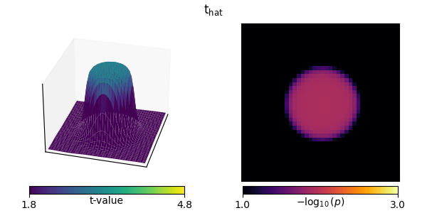
“hat”技术对 t 检验计算中使用的方差值进行正则化 [1]，以补偿小得不合理的方差。

ts.append(ttest_1samp_no_p(X, sigma=sigma))
ps.append(stats.distributions.t.sf(np.abs(ts[-1]), len(X) - 1) * 2)
titles.append(r"$\mathrm{t_{hat}}$")
mccs.append(假)
plot_t_p(ts[-1], ps[-1], titles[-1], mccs[-1])

$\mathrm{t_{hat}}$

非参数检验#

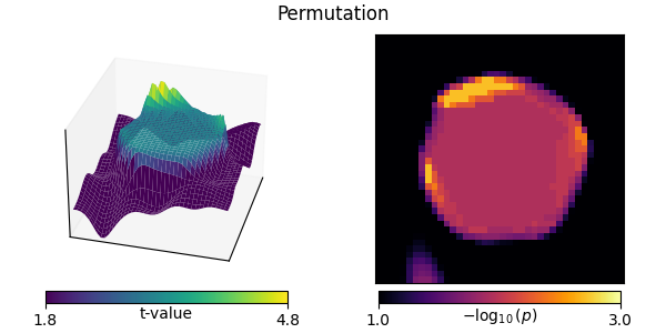
与其假定潜在的高斯分布，我们也可以改用非参数重采样方法。对于条件 A 与 B 之间的配对 t 检验（在数学上等价于对条件差值 A-B 做单样本 t 检验），在零假设下我们可利用可交换性（exchangeability）原理。这意味着，如果零假设为真，我们可以交换条件而不改变检验统计量的分布。

因此，在使用配对 t 检验时，可交换性意味着我们可以翻转 A 与 B 之间差值的符号。于是，我们可以通过对样本（受试者）随机取子集、翻转其差值的符号，并记录所得统计量的绝对值（之所以记录绝对值，是因为我们进行双尾检验），来为每个体素构造零分布值。然后可将真实数据上评估得到的统计量绝对值与该分布比较，p 值就是更小的零分布值所占的比例。

警告

对于真正的单样本 t 检验，即分析单个条件而非两个条件之间的差异时，可交换性在何处以及如何适用并不明确；参见这篇 FieldTrip 讨论。

当 n_permutations 足够大（或设为 “all”），从而可以完成全部唯一的重采样交换时（单尾检验为 $2^{N_{samp}}-1$ 种，双尾检验为 $2^{N_{samp}-1}-1$ 种，不计真实分布本身），零分布不再由随机交换条件构造，而是使用所有可能的交换来形成。这称为置换检验（permutation test，或称精确检验 exact test）。

# Here we have to do a bit of gymnastics to get our function to do
# a permutation test without correcting for multiple comparisons:

X = X.reshape(n_subjects, n_src)  # flatten the array for simplicity
titles.append("Permutation")
ts.append(np.zeros(width * width))
ps.append(np.zeros(width * width))
mccs.append(假)
for ii in range(n_src):
    t, p = permutation_t_test(X[:, [ii]], verbose=假, rng=47)[:2]
    ts[-1][ii], ps[-1][ii] = t[0], p[0]
plot_t_p(ts[-1], ps[-1], titles[-1], mccs[-1])

多重比较#

到目前为止，我们尚未对多重比较做任何校正。这对当前数据可能是个问题，因为共进行了 $40 \cdot 40 = 1600$ 次检验。如果对每次单独检验都使用 p < 0.05 的阈值，那么即使不存在真实效应，我们也会预期许多体素被判定为显著。换言之，我们会犯许多第一类错误（改编自此处）：

		零假设
		真	假
拒绝	是	第一类错误假阳性	正确真阳性
拒绝	No	正确真阴性	第二类错误假阴性

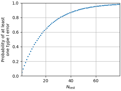
为说明原因，考虑标准的 $\alpha = 0.05$。对于单次检验，犯第一类错误的概率是 0.05。那么在 $N_{\mathrm{test}}$ 次独立检验中至少犯一次第一类错误的概率为 $1 - (1 - \alpha)^{N_{\mathrm{test}}}$：

N = np.arange(1, 80)
alpha = 0.05
p_type_I = 1 - (1 - alpha) ** N
fig, ax = plt.subplots(figsize=(4, 3), layout="constrained")
ax.scatter(N, p_type_I, 3)
ax.set(
    xlim=N[[0, -1]],
    ylim=[0, 1],
    xlabel=r"$N_{\mathrm{test}}$",
    ylabel="Probability of at least\none type I error",
)
ax.grid(真)
fig.show()

为应对这一问题，存在多种方法。通常这些方法控制以下两种指标之一：

族错误率（FWER）
犯一次或多次第一类错误的概率：\[\mathrm{P}(N_{\mathrm{type\ I}} >= 1 \mid H_0)\]
错误发现率（FDR）
被拒绝的零假设中实际为真的期望比例：\[\mathrm{E}(\frac{N_{\mathrm{type\ I}}}{N_{\mathrm{reject}}} \mid N_{\mathrm{reject}} > 0) \cdot \mathrm{P}(N_{\mathrm{reject}} > 0 \mid H_0)\]

下面我们介绍一些控制 FWER 和 FDR 的技术。

Bonferroni 校正#

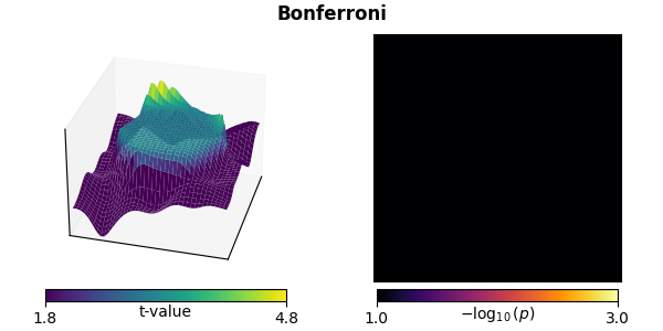
Bonferroni 校正或许是处理多重比较最简单的方法，它保守地将 p 值乘以比较次数，以控制 FWER。

titles.append("Bonferroni")
ts.append(ts[-1])
ps.append(bonferroni_correction(ps[0])[1])
mccs.append(真)
plot_t_p(ts[-1], ps[-1], titles[-1], mccs[-1])

错误发现率（FDR）校正#

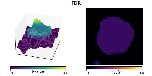
FDR 通常通过 Benjamini-Hochberg 过程实现。在比较次数较多时，它比 Bonferroni 校正限制更少（第二类错误更少），但对第一类错误的控制不那么严格。

titles.append("FDR")
ts.append(ts[-1])
ps.append(fdr_correction(ps[0])[1])
mccs.append(真)
plot_t_p(ts[-1], ps[-1], titles[-1], mccs[-1])

基于最大统计量的非参数重采样检验#

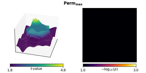
非参数重采样检验也可用于校正多重比较。在最简单的形式中，我们同样在零假设下利用可交换性进行置换，但这次在每次置换中取所有体素上的最大统计量来构成零分布。然后，真实数据中每个体素的 p 值就是更小的零分布值所占的比例。

该方法有两个重要特点：

它控制 FWER。
它是非参数的。尽管初始检验统计量（这里是单样本 t 检验）是参数的，但用于拒绝零假设（各受试者的均值与零无法区分）的零分布是通过置换得到的。这意味着它不对高斯性做任何假设（本示例确实满足高斯性，但对某些类型的处理后神经影像数据而言通常并不满足）。

titles.append(r"$\mathbf{Perm_{max}}$")
out = permutation_t_test(X, verbose=假, rng=53)[:2]
ts.append(out[0])
ps.append(out[1])
mccs.append(真)
plot_t_p(ts[-1], ps[-1], titles[-1], mccs[-1])

$\mathbf{Perm_{max}}$

聚类#

上述每一种多重比较校正的缺点都是没有充分纳入数据的相关结构，即彼此靠近的点（例如在空间或时间上）往往存在相关。然而，通过在我们的数据中定义邻接（或“邻居”）结构，我们可以利用聚类来进行补偿。

要使用这一方法，我们需要重新思考零假设。我们不再考虑关于每个体素均值的零假设（每个体素一次独立检验），而是考虑关于数据中簇大小的零假设，可以表述为：

在两种实验条件下观察到的空间簇大小分布来自同一概率分布。

这里我们只有一个条件，并将其与零对比，可以理解为：

空间簇大小的分布与数据的符号无关。

在这种情况下，我们同样使用最大统计量进行置换，但在每次置换中，我们：

单独计算每个体素的检验统计量。
对检验统计量值进行阈值化。
根据邻接关系，将超过该阈值（且符号相同）的体素聚成簇。
保留最大簇的大小（例如用简单的体素计数，或用簇内体素 t 值之和来度量），以构建零分布。

完成这些置换后，将真实数据中的簇大小与该零分布比较。每个簇对应的 p 值同样是更小的零分布值所占的比例。随后可对其应用标准的 p 值阈值（例如 p < 0.05）来拒绝零假设（即找到感兴趣的效应）。

这种改为考虑簇大小而非单个均值的思路，保留了标准非参数置换检验的优点——即控制 FWER 且不对参数数据分布做假设。但关键的是，它还考虑了数据中的相关结构——在这个玩具示例中是空间相关，但一般而言可以是多维的（例如时空相关）——因为零分布将以保留这些相关性的方式从数据中导出。

效应量

关于如何计算聚类检验中得到的效应量，参见这篇 FieldTrip 邮件列表讨论。

然而，这也有一个缺点。如果某个簇显著偏离零假设，就无法再对该簇做进一步推断（例如峰值位置），因为拒绝零假设时是把整个簇作为一个整体。此外，由于检验统计量涉及全部数据，零假设（以及我们对它的拒绝）指向的是全部数据的结构。更多信息另见这份全面的 FieldTrip 教程。

定义邻接矩阵#

首先我们需要定义邻接（有时称为“邻居”）矩阵。这是一个形状为 (n_src, n_src) 的方阵（或稀疏矩阵），包含 0 和 1，用于定义哪些空间点是邻居，即哪些体素彼此相邻。在我们的情形中这相当简单，因为数据对齐在矩形网格上。

假设我们的数据更小——一个 3 × 3 的网格。若把每个体素视为与它接触到的其他体素相连，我们需要一个 9 × 9 的邻接矩阵。该矩阵的第一行包含展平后数据中第一个体素所接触的体素。由于它接触第一行的第二个元素和第二行的第一个元素（并且也是自身的邻居），因此为：

[1, 1, 0, 1, 0, 0, 0, 0, 0]

sklearn.feature_extraction 为此提供了一个便捷函数：

from sklearn.feature_extraction.image import grid_to_graph  # noqa: E402

mini_adjacency = grid_to_graph(3, 3).toarray()
assert mini_adjacency.shape == (9, 9)
print(mini_adjacency[0])

[1 1 0 1 0 0 0 0 0]

一般而言，体素之间的邻接关系可能更复杂，例如 3D 空间中传感器之间的邻接，或皮层表面上脑顶点处随时间变化的激活。MNE 提供了若干计算邻接矩阵的便捷函数，例如：

完整列表参见 Statistics API。

MNE 还内置了来自 FieldTrip 项目的大量通道邻接矩阵（在那里称为“neighbors”）。你可以使用 mne.channels.get_builtin_ch_adjacencies() 查看它们的概览：

builtin_ch_adj = mne.channels.get_builtin_ch_adjacencies(descriptions=真)
for adj_name, adj_description in builtin_ch_adj:
    print(f"{adj_name}: {adj_description}")

biosemi16: Biosemi 16-electrode cap
biosemi32: Biosemi 32-electrode cap
biosemi64: Biosemi 64-electrode cap
bti148: BTI 148-channel system
bti248: BTI 248-channel system
bti248grad: BTI 248 gradiometer system
ctf151: CTF 151 axial gradiometer
ctf275: CTF 275 axial gradiometer
ctf64: CTF 64 axial gradiometer
easycap128ch-avg:
easycap32ch-avg:
easycap64ch-avg:
easycapM1: Easycap M1
easycapM11: Easycap M11
easycapM14: Easycap M14
easycapM15: Easycap M15
ecog256: ECOG 256channels, average referenced
ecog256bipolar: ECOG 256channels, bipolar referenced
eeg1010_neighb:
elec1005: Standard 10-05 system
elec1010: Standard 10-10 system
elec1020: Standard 10-20 system
itab153: ITAB 153-channel system
itab28: ITAB 28-channel system
KIT-157:
KIT-208:
KIT-NYU-2019:
KIT-UMD-1:
KIT-UMD-2:
KIT-UMD-3:
KIT-UMD-4:
language29ch-avg: MPI for Psycholinguistic: Averaged 29-channel cap
mpi_59_channels: MPI for Psycholinguistic: 59-channel cap
neuromag122cmb: Neuromag122, only combined planar gradiometers
neuromag306cmb: Neuromag306, only combined planar gradiometers
neuromag306mag: Neuromag306, only magnetometers
neuromag306planar: Neuromag306, only planar gradiometers
yokogawa160:
yokogawa440:

这些内置通道邻接矩阵可通过 mne.channels.read_ch_adjacency() 加载。

标准聚类#

这里由于我们的数据位于网格上，可以使用 adjacency=None 触发优化的网格代码，并运行聚类算法。

titles.append("聚类")

# Reshape data to what is equivalent to (n_samples, n_space, n_time)
X = X.reshape(n_subjects, width, width)

# Compute threshold from t distribution (this is also the default)
# Here we use a two-tailed test, hence we need to divide alpha by 2.
# Subtracting alpha from 1 guarantees that we get a positive threshold,
# which MNE-Python expects for two-tailed tests.
df = n_subjects - 1  # degrees of freedom
t_thresh = stats.distributions.t.ppf(1 - alpha / 2, df=df)

# run the cluster test
t_clust, clusters, p_values, H0 = permutation_cluster_1samp_test(
    X,
    rng=59,
    n_jobs=None,
    threshold=t_thresh,
    adjacency=None,
    n_permutations=n_permutations,
    out_type="mask",
)

# Put the cluster data in a viewable format
p_clust = np.ones((width, width))
for cl, p in zip(clusters, p_values):
    p_clust[cl] = p
ts.append(t_clust)
ps.append(p_clust)
mccs.append(真)
plot_t_p(ts[-1], ps[-1], titles[-1], mccs[-1])

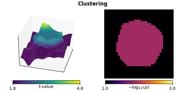
stat_fun(H1): min=-1.358953936098723 max=5.977484949679637
Running initial clustering …
Found 2 clusters

  0%|          | Permuting : 0/510 [00:00<?,       ?it/s]
 96%|█████████▌| Permuting : 490/510 [00:00<00:00, 14536.46it/s]
100%|██████████| Permuting : 510/510 [00:00<00:00, 14391.02it/s]

“hat”方差校正#

该方法在此情境下也可用于校正小方差 [1]：

titles.append(r"$\mathbf{C_{hat}}$")
stat_fun_hat = partial(ttest_1samp_no_p, sigma=sigma)
t_hat, clusters, p_values, H0 = permutation_cluster_1samp_test(
    X,
    rng=61,
    n_jobs=None,
    threshold=t_thresh,
    adjacency=None,
    out_type="mask",
    n_permutations=n_permutations,
    stat_fun=stat_fun_hat,
    buffer_size=None,
)
p_hat = np.ones((width, width))
for cl, p in zip(clusters, p_values):
    p_hat[cl] = p
ts.append(t_hat)
ps.append(p_hat)
mccs.append(真)
plot_t_p(ts[-1], ps[-1], titles[-1], mccs[-1])

$\mathbf{C_{hat}}$

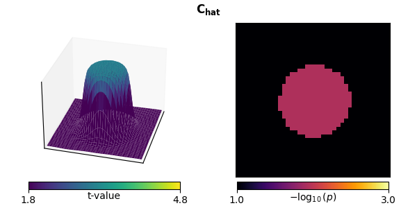
stat_fun(H1): min=-0.031063870537674506 max=4.257794505612697
Running initial clustering …
Found 1 cluster

  0%|          | Permuting : 0/510 [00:00<?,       ?it/s]
100%|██████████| Permuting : 510/510 [00:00<00:00, 17004.48it/s]
100%|██████████| Permuting : 510/510 [00:00<00:00, 16911.45it/s]

无阈值聚类增强（TFCE）#

TFCE 消除了决定哪些点纳入聚类的自由参数初始阈值，其方法是用标准黎曼和 [2] 对可能的阈值做连续积分近似。这需要给出起始阈值 start 和步长 step，在 MNE 中以 dict 形式提供。步长越小、start 越接近 0，近似越好，但耗时越长。

TFCE 的一个显著优势在于，它并不改变所检验的统计零假设（从关于单个体素变为关于数据中簇的分布），而是在仍然控制多重比较的同时改变所检验的数据。这样统计检验就在单个体素层面而非簇层面进行。这使得可以独立评估每个点的显著性，而不只是将其作为簇组来评估。

titles.append(r"$\mathbf{C_{TFCE}}$")
threshold_tfce = dict(start=0, step=0.2)
t_tfce, _, p_tfce, H0 = permutation_cluster_1samp_test(
    X,
    rng=67,
    n_jobs=None,
    threshold=threshold_tfce,
    adjacency=None,
    n_permutations=n_permutations,
    out_type="mask",
)
ts.append(t_tfce)
ps.append(p_tfce)
mccs.append(真)
plot_t_p(ts[-1], ps[-1], titles[-1], mccs[-1])

$\mathbf{C_{TFCE}}$

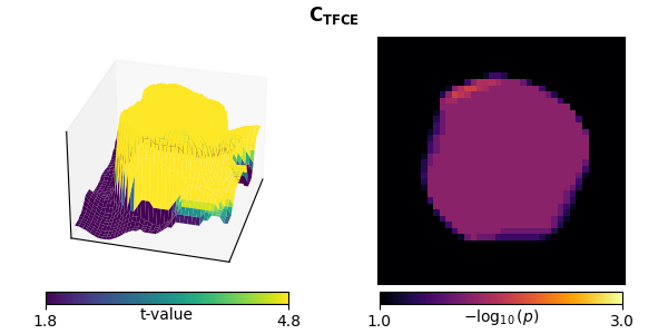
stat_fun(H1): min=-1.358953936098723 max=5.977484949679637
Running initial clustering …
Using 30 thresholds from 0.00 to 5.80 for TFCE computation (h_power=2.00, e_power=0.50)
Found 1600 clusters

  0%|          | Permuting : 0/510 [00:00<?,       ?it/s]
  5%|▍         | Permuting : 23/510 [00:00<00:00,  662.35it/s]
  9%|▉         | Permuting : 47/510 [00:00<00:00,  688.81it/s]
 14%|█▎        | Permuting : 70/510 [00:00<00:00,  687.62it/s]
 18%|█▊        | Permuting : 93/510 [00:00<00:00,  687.08it/s]
 23%|██▎       | Permuting : 116/510 [00:00<00:00,  686.80it/s]
 28%|██▊       | Permuting : 141/510 [00:00<00:00,  697.77it/s]
 32%|███▏      | Permuting : 163/510 [00:00<00:00,  690.84it/s]
 37%|███▋      | Permuting : 187/510 [00:00<00:00,  694.50it/s]
 41%|████      | Permuting : 210/510 [00:00<00:00,  692.89it/s]
 46%|████▌     | Permuting : 234/510 [00:00<00:00,  695.69it/s]
 50%|█████     | Permuting : 257/510 [00:00<00:00,  692.33it/s]
 55%|█████▍    | Permuting : 280/510 [00:00<00:00,  691.57it/s]
 60%|█████▉    | Permuting : 305/510 [00:00<00:00,  697.06it/s]
 64%|██████▍   | Permuting : 328/510 [00:00<00:00,  695.95it/s]
 69%|██████▉   | Permuting : 351/510 [00:00<00:00,  695.00it/s]
 73%|███████▎  | Permuting : 372/510 [00:00<00:00,  688.83it/s]
 77%|███████▋  | Permuting : 395/510 [00:00<00:00,  687.35it/s]
 82%|████████▏ | Permuting : 420/510 [00:00<00:00,  692.10it/s]
 87%|████████▋ | Permuting : 443/510 [00:00<00:00,  691.56it/s]
 92%|█████████▏| Permuting : 467/510 [00:00<00:00,  693.40it/s]
 96%|█████████▋| Permuting : 491/510 [00:00<00:00,  695.04it/s]
100%|██████████| Permuting : 510/510 [00:00<00:00,  697.22it/s]
100%|██████████| Permuting : 510/510 [00:00<00:00,  695.17it/s]

我们也可以把 TFCE 与“hat”校正结合使用：

titles.append(r"$\mathbf{C_{hat,TFCE}}$")
t_tfce_hat, _, p_tfce_hat, H0 = permutation_cluster_1samp_test(
    X,
    rng=71,
    n_jobs=None,
    threshold=threshold_tfce,
    adjacency=None,
    out_type="mask",
    n_permutations=n_permutations,
    stat_fun=stat_fun_hat,
    buffer_size=None,
)
ts.append(t_tfce_hat)
ps.append(p_tfce_hat)
mccs.append(真)
plot_t_p(ts[-1], ps[-1], titles[-1], mccs[-1])

$\mathbf{C_{hat,TFCE}}$

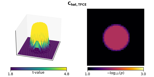
stat_fun(H1): min=-0.031063870537674506 max=4.257794505612697
Running initial clustering …
Using 22 thresholds from 0.00 to 4.20 for TFCE computation (h_power=2.00, e_power=0.50)
Found 1600 clusters

  0%|          | Permuting : 0/510 [00:00<?,       ?it/s]
 22%|██▏       | Permuting : 110/510 [00:00<00:00, 3121.94it/s]
 44%|████▎     | Permuting : 222/510 [00:00<00:00, 3229.38it/s]
 63%|██████▎   | Permuting : 323/510 [00:00<00:00, 3153.68it/s]
 84%|████████▎ | Permuting : 427/510 [00:00<00:00, 3138.80it/s]
100%|██████████| Permuting : 510/510 [00:00<00:00, 3148.38it/s]
100%|██████████| Permuting : 510/510 [00:00<00:00, 3146.37it/s]

可视化并比较各方法#

让我们看看这些统计结果。上排显示各检验统计量，下排显示各种统计检验的 p 值，其中对 FWER 或 FDR 有恰当控制的检验以粗体标题标出。

fig = plt.figure(facecolor="w", figsize=(14, 3), layout="constrained")
assert len(ts) == len(titles) == len(ps)
for ii in range(len(ts)):
    ax = [
        fig.add_subplot(2, 10, ii + 1, projection="3d"),
        fig.add_subplot(2, 10, 11 + ii),
    ]
    plot_t_p(ts[ii], ps[ii], titles[ii], mccs[ii], ax)

$t, $\mathrm{t_{hat}}$, Permutation, Bonferroni, FDR, $\mathbf{Perm_{max}}$, Clustering, $\mathbf{C_{hat}}$, $\mathbf{C_{TFCE}}$, $\mathbf{C_{hat,TFCE}}$$

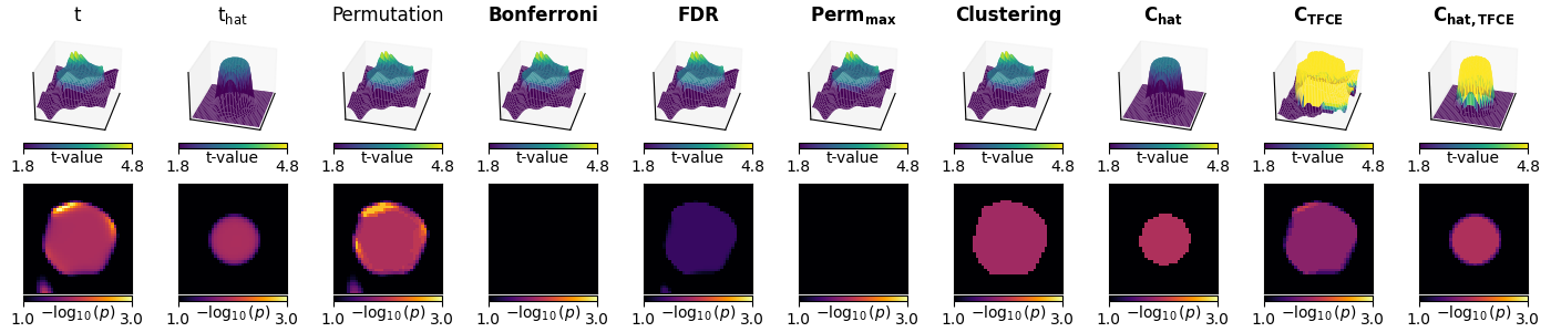
前三列显示未对多重比较校正的参数与非参数统计量：

质量单变量 t 检验会产生锯齿状边缘。
对 t 检验进行“hat”方差校正后，边缘的尖峰减弱，从而校正了由低方差体素导致的统计量尖锐性。
非参数重采样检验与 t 检验非常相似。这是意料之中的：数据来自高斯分布，因而满足参数假设。

接下来三列显示对质量单变量检验（参数与非参数）的多重比较校正。由于我们数据中相邻体素存在相关，这些校正同样过于保守：

Bonferroni 校正消除了所有显著活动。
FDR 校正比 Bonferroni 保守程度低。
使用最大统计量的置换检验也消除了所有显著活动。

最后四列显示使用最大统计量的非参数基于簇的置换检验：

标准聚类识别出了正确的区域。然而必须把整个区域判定为显著，因此无法进行峰值分析。此外，峰值较宽。
使用“hat”方差调整的聚类使显著活动的估计更紧致。
使用 TFCE 的聚类允许独立分析每个显著点，但估计结果仍然偏宽。
结合 TFCE 与“hat”方差调整的聚类使判定为显著的区域更紧致（同样经过 FWER 校正）。

MNE 中的统计函数#

MNE 提供的统计函数完整列表见 Statistics API 列表，这里我们做一简要概述。

MNE 提供了若干便捷的参数检验函数，可与非参数聚类方法配合使用。不过，我们提供的函数集合并非力求详尽。

如果这里没有列出你感兴趣的单变量统计对比（例如非平衡 ANOVA 中的交互项），可以考虑查看 statsmodels 包。它提供了许多计算统计对比的函数，例如 statsmodels.stats.anova.anova_lm()。要在聚类中使用这些函数：

确定你会在单变量情境中使用哪种检验统计量（例如 t 值、F 值）来计算感兴趣的对比。换言之，如果只有一个输出（例如反应时），你会对数据计算什么检验统计量？
将对该函数的调用包装在一个函数中：该函数接受与聚类函数期望相同形状的输入，并返回一个去掉“samples”维度后形状相同的数组（例如 mne.stats.permutation_cluster_1samp_test() 接受形状为 (n_samples, p, q) 的数组，并返回形状为 (p, q) 的数组）。
将这个包装后的函数传给聚类函数的 stat_fun 参数。
根据你的统计对比函数返回的值，设置合适的阈值（float 或 dict）。

MNE 提供的参数方法#

mne.stats.ttest_1samp_no_p()
配对 t 检验，可选 hat 调整。默认用于配对聚类检验中的对比增强。
mne.stats.f_oneway()
独立样本的单因素方差分析。可用于计算各种 F 对比。默认用于非配对聚类检验中的对比增强。
mne.stats.f_mway_rm()
用于重复测量且设计平衡的 M 因素方差分析。返回 F 统计量和 p 值。相关的辅助函数 mne.stats.f_threshold_mway_rm() 可用于确定给定显著性水平下的 F 阈值。
mne.stats.linear_regression()
对多个目标（例如传感器、跨试次的时间点（样本））计算普通最小二乘回归。对每个回归量，它返回 beta 值、t 统计量和未校正的 p 值。虽然它可用作检验，但尤其适用于计算加权平均或处理连续预测变量。

非参数方法#

mne.stats.permutation_cluster_test()
带聚类的非配对对比。
mne.stats.spatio_temporal_cluster_test()
带时空聚类的非配对对比。
mne.stats.permutation_t_test()
不带聚类的配对对比。
mne.stats.permutation_cluster_1samp_test()
带聚类的配对对比。
mne.stats.spatio_temporal_cluster_1samp_test()
带时空聚类的配对对比。

警告

在大多数 MNE 函数中，数据的形状为 (..., n_space, n_time)，其中空间维度可以是传感器或源顶点等。但对于我们的时空聚类函数，出于计算效率的考虑，空间维度需要放在最后。例如，对于 mne.stats.spatio_temporal_cluster_1samp_test()，X 的形状需要是 (n_samples, n_time, n_space)。如有必要，可以使用 numpy.transpose() 转置轴。

参考文献#

脚本总运行时间：（0 分钟 3.843 秒）

图库由 Sphinx-Gallery 生成