
非官方中文翻译
本页译自 MNE-Python 官方文档:
查看英文原文 ↗。
文档版权归 MNE Developers 所有(BSD-3-Clause)。
说明
转到末尾下载完整示例代码。
从源估计生成功能标签#
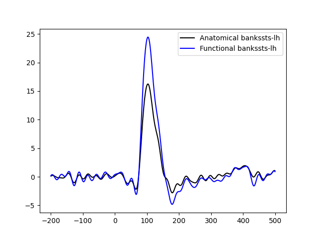
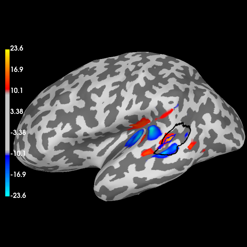
对源估计做阈值处理并生成功能标签。标签通常是包含高值的感兴趣区域。这里比较由 FreeSurfer 分割得到的解剖标签中的平均时间过程与功能标签的平均时间过程。正如预期,功能标签中的时间过程给出更高的数值。
# Author: Luke Bloy <luke.bloy@gmail.com>
#         Alex Gramfort <alexandre.gramfort@inria.fr>
# License: BSD-3-Clause
# Copyright the MNE-Python contributors.
import matplotlib.pyplot as plt
import numpy as np

import mne
from mne.datasets import sample
from mne.minimum_norm import apply_inverse, read_inverse_operator

print(__doc__)

data_path = sample.data_path()
fname_inv = data_path / "MEG" / "sample" / "sample_audvis-meg-oct-6-meg-inv.fif"
fname_evoked = data_path / "MEG" / "sample" / "sample_audvis-ave.fif"
subjects_dir = data_path / "subjects"
subject = "sample"

snr = 3.0
lambda2 = 1.0 / snr**2
method = "dSPM"  # use dSPM method (could also be MNE or sLORETA)

# Compute a label/ROI based on the peak power between 80 and 120 ms.
# The label bankssts-lh is used for the comparison.
aparc_label_name = "bankssts-lh"
tmin, tmax = 0.080, 0.120

# Load data
evoked = mne.read_evokeds(fname_evoked, condition=0, baseline=(None, 0))
inverse_operator = read_inverse_operator(fname_inv)
src = inverse_operator["src"]  # get the source space

# Compute inverse solution
stc = apply_inverse(evoked, inverse_operator, lambda2, method, pick_ori="normal")

# Make an STC in the time interval of interest and take the mean
stc_mean = stc.copy().crop(tmin, tmax).mean()

# use the stc_mean to generate a functional label
# region growing is halted at 60% of the peak value within the
# anatomical label / ROI specified by aparc_label_name
label = mne.read_labels_from_annot(
    subject, parc="aparc", subjects_dir=subjects_dir, regexp=aparc_label_name
)[0]
stc_mean_label = stc_mean.in_label(label)
data = np.abs(stc_mean_label.data)
stc_mean_label.data[data < 0.6 * np.max(data)] = 0.0

# 8.5% of original source space vertices were omitted during forward
# calculation, suppress the warning here with verbose='error'
func_labels, _ = mne.stc_to_label(
    stc_mean_label,
    src=src,
    smooth=True,
    subjects_dir=subjects_dir,
    connected=True,
    verbose="error",
)

# take first as func_labels are ordered based on maximum values in stc
func_label = func_labels[0]

# load the anatomical ROI for comparison
anat_label = mne.read_labels_from_annot(
    subject, parc="aparc", subjects_dir=subjects_dir, regexp=aparc_label_name
)[0]

# extract the anatomical time course for each label
stc_anat_label = stc.in_label(anat_label)
pca_anat = stc.extract_label_time_course(anat_label, src, mode="pca_flip")[0]

stc_func_label = stc.in_label(func_label)
pca_func = stc.extract_label_time_course(func_label, src, mode="pca_flip")[0]

# flip the pca so that the max power between tmin and tmax is positive
pca_anat *= np.sign(pca_anat[np.argmax(np.abs(pca_anat))])
pca_func *= np.sign(pca_func[np.argmax(np.abs(pca_anat))])
Reading /home/circleci/mne_data/MNE-sample-data/MEG/sample/sample_audvis-ave.fif ...
    Read a total of 4 projection items:
        PCA-v1 (1 x 10²) active
        PCA-v2 (1 x 10²) active
        PCA-v3 (1 x 10²) active
        Average EEG reference (1 x 60) active
    Found the data of interest:
        t =    -199.80 ...     499.49 ms (Left Auditory)
        0 CTF compensation matrices available
        nave = 55 - aspect type = 100
Projections have already been applied. Setting proj attribute to True.
Applying baseline correction (mode: mean)
Reading inverse operator decomposition from /home/circleci/mne_data/MNE-sample-data/MEG/sample/sample_audvis-meg-oct-6-meg-inv.fif...
    Reading inverse operator info...
    [done]
    Reading inverse operator decomposition...
    [done]
    305 x 305 full covariance (kind = 1) found.
    Read a total of 4 projection items:
        PCA-v1 (1 x 10²) active
        PCA-v2 (1 x 10²) active
        PCA-v3 (1 x 10²) active
        Average EEG reference (1 x 60) active
    Noise covariance matrix read.
    22494 x 22494 diagonal covariance (kind = 2) found.
    Source covariance matrix read.
    22494 x 22494 diagonal covariance (kind = 6) found.
    Orientation priors read.
    22494 x 22494 diagonal covariance (kind = 5) found.
    Depth priors read.
    Did not find the desired covariance matrix (kind = 3)
    Reading a source space...
    Computing patch statistics...
    Patch information added...
    Distance information added...
    [done]
    Reading a source space...
    Computing patch statistics...
    Patch information added...
    Distance information added...
    [done]
    2 source spaces read
    Read a total of 4 projection items:
        PCA-v1 (1 x 10²) active
        PCA-v2 (1 x 10²) active
        PCA-v3 (1 x 10²) active
        Average EEG reference (1 x 60) active
    Source spaces transformed to the inverse solution coordinate frame
Preparing the inverse operator for use...
    Scaled noise and source covariance from nave = 1 to nave = 55
    Created the regularized inverter
    Created an SSP operator (subspace dimension = 3)
    Created the whitener using a noise covariance matrix with rank 302 (3 small eigenvalues omitted)
    Computing noise-normalization factors (dSPM)...
[done]
Applying inverse operator to "Left Auditory"...
    Picked 305 channels from the data
    Computing inverse...
    Eigenleads need to be weighted ...
    Computing residual...
    Explained  59.4% variance
    dSPM...
[done]
Reading labels from parcellation...
   read 1 labels from /home/circleci/mne_data/MNE-sample-data/subjects/sample/label/lh.aparc.annot
   read 0 labels from /home/circleci/mne_data/MNE-sample-data/subjects/sample/label/rh.aparc.annot
Reading labels from parcellation...
   read 1 labels from /home/circleci/mne_data/MNE-sample-data/subjects/sample/label/lh.aparc.annot
   read 0 labels from /home/circleci/mne_data/MNE-sample-data/subjects/sample/label/rh.aparc.annot
Extracting time courses for 1 labels (mode: pca_flip)
Extracting time courses for 1 labels (mode: pca_flip)
绘制时间过程……
plt.figure()
plt.plot(
    1e3 * stc_anat_label.times, pca_anat, "k", label=f"Anatomical {aparc_label_name}"
)
plt.plot(
    1e3 * stc_func_label.times, pca_func, "b", label=f"Functional {aparc_label_name}"
)
plt.legend()
plt.show()
若可用,使用 mne.viz.Brain 以 3D 绘制大脑
brain = stc_mean.plot(hemi="lh", subjects_dir=subjects_dir)
brain.show_view("lateral")

# show both labels
brain.add_label(anat_label, borders=True, color="k")
brain.add_label(func_label, borders=True, color="b")
Using control points [ 8.73227205 10.80078852 23.62750681]
脚本总运行时间:(0 分 2.710 秒)