
非官方中文翻译
本页译自 MNE-Python 官方文档:
查看英文原文 ↗。
文档版权归 MNE Developers 所有(BSD-3-Clause)。
说明
转到末尾下载完整示例代码。
计算多种 MNE 解#
本示例展示了由 MNE-Python 中实现的最小范数变体生成的固定朝向与自由朝向源定位结果:MNE、dSPM、sLORETA 和 eLORETA。
# Author: Eric Larson <larson.eric.d@gmail.com>
#
# License: BSD-3-Clause
# Copyright the MNE-Python contributors.
import mne
from mne.datasets import sample
from mne.minimum_norm import apply_inverse, apply_inverse_cov, make_inverse_operator

print(__doc__)

data_path = sample.data_path()
subjects_dir = data_path / "subjects"

# Read data (just MEG here for speed, though we could use MEG+EEG)
meg_path = data_path / "MEG" / "sample"
fname_evoked = meg_path / "sample_audvis-ave.fif"
evoked = mne.read_evokeds(fname_evoked, condition="Right Auditory", baseline=(None, 0))
fname_fwd = meg_path / "sample_audvis-meg-oct-6-fwd.fif"
fname_cov = meg_path / "sample_audvis-cov.fif"
fwd = mne.read_forward_solution(fname_fwd)
cov = mne.read_cov(fname_cov)
# crop for speed in these examples
evoked.crop(0.05, 0.15)
Reading /home/circleci/mne_data/MNE-sample-data/MEG/sample/sample_audvis-ave.fif ...
    Read a total of 4 projection items:
        PCA-v1 (1 x 10²) active
        PCA-v2 (1 x 10²) active
        PCA-v3 (1 x 10²) active
        Average EEG reference (1 x 60) active
    Found the data of interest:
        t =    -199.80 ...     499.49 ms (Right Auditory)
        0 CTF compensation matrices available
        nave = 61 - aspect type = 100
Projections have already been applied. Setting proj attribute to True.
Applying baseline correction (mode: mean)
Reading forward solution from /home/circleci/mne_data/MNE-sample-data/MEG/sample/sample_audvis-meg-oct-6-fwd.fif...
    Reading a source space...
    Computing patch statistics...
    Patch information added...
    Distance information added...
    [done]
    Reading a source space...
    Computing patch statistics...
    Patch information added...
    Distance information added...
    [done]
    2 source spaces read
    Desired named matrix (kind = 3523 (FIFF_MNE_FORWARD_SOLUTION_GRAD)) not available
    Read MEG forward solution (7498 sources, 306 channels, free orientations)
    Source spaces transformed to the forward solution coordinate frame
    366 x 366 full covariance (kind = 1) found.
    Read a total of 4 projection items:
        PCA-v1 (1 x 10²) active
        PCA-v2 (1 x 10²) active
        PCA-v3 (1 x 10²) active
        Average EEG reference (1 x 60) active
固定朝向#
首先,我们使用默认权重创建一个固定朝向的逆算子。
inv = make_inverse_operator(evoked.info, fwd, cov, loose=0.0, depth=0.8, verbose=True)
Computing inverse operator with 305 channels.
    305 out of 306 channels remain after picking
Selected 305 channels
Creating the depth weighting matrix...
    203 planar channels
    limit = 7265/7498 = 10.037797
    scale = 2.52065e-08 exp = 0.8
    Picked elements from a free-orientation depth-weighting prior into the fixed-orientation one
    Average patch normals will be employed in the rotation to the local surface coordinates....
    Converting to surface-based source orientations...
    [done]
Whitening the forward solution.
    Created an SSP operator (subspace dimension = 3)
Computing rank from covariance with rank=None
    Using tolerance 3.3e-13 (2.2e-16 eps * 305 dim * 4.8  max singular value)
    Estimated rank (mag + grad): 302
    MEG: rank 302 computed from 305 data channels with 3 projectors
    Setting small MEG eigenvalues to zero (without PCA)
Creating the source covariance matrix
Adjusting source covariance matrix.
Computing SVD of whitened and weighted lead field matrix.
    largest singular value = 4.65922
    scaling factor to adjust the trace = 6.72259e+18 (nchan = 305 nzero = 3)
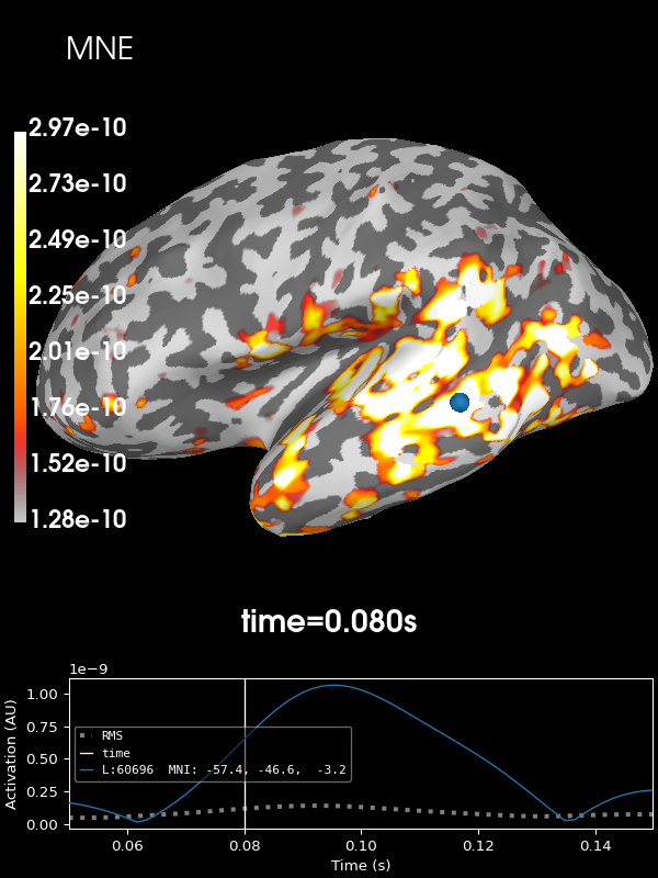
让我们用 MNE 查看当前估计。为简化可视化,我们将取源估计的绝对值。
snr = 3.0
lambda2 = 1.0 / snr**2
kwargs = dict(
    initial_time=0.08,
    hemi="lh",
    subjects_dir=subjects_dir,
    size=(600, 600),
    clim=dict(kind="percent", lims=[90, 95, 99]),
    smoothing_steps=10,
)

stc = abs(apply_inverse(evoked, inv, lambda2, "MNE", verbose=True))
brain = stc.plot(**kwargs)
brain.add_text(0.1, 0.9, "MNE", "title", font_size=14)
Preparing the inverse operator for use...
    Scaled noise and source covariance from nave = 1 to nave = 61
    Created the regularized inverter
    Created an SSP operator (subspace dimension = 3)
    Created the whitener using a noise covariance matrix with rank 302 (3 small eigenvalues omitted)
Applying inverse operator to "Right Auditory"...
    Picked 305 channels from the data
    Computing inverse...
    Eigenleads need to be weighted ...
    Computing residual...
    Explained  78.4% variance
[done]
Using control points [1.28047949e-10 1.72734062e-10 2.97200565e-10]
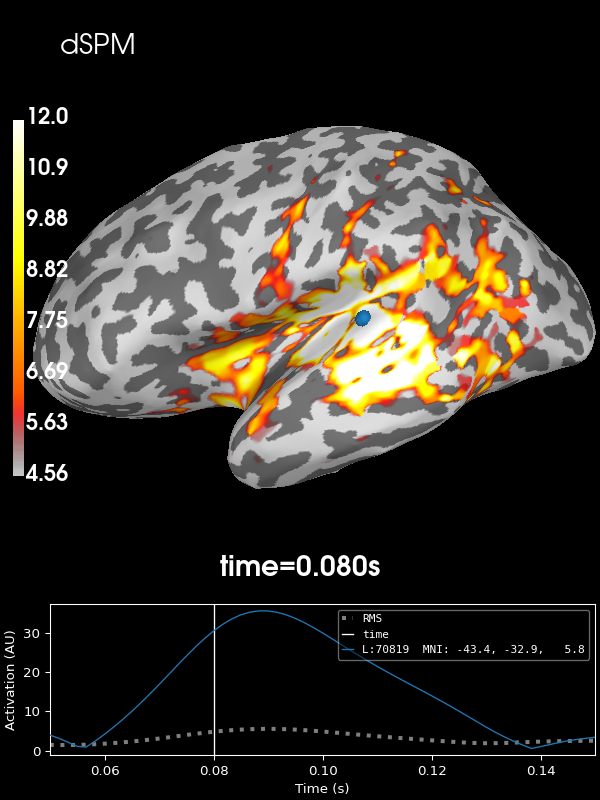
接下来使用默认的噪声归一化方法 dSPM:
stc = abs(apply_inverse(evoked, inv, lambda2, "dSPM", verbose=True))
brain = stc.plot(**kwargs)
brain.add_text(0.1, 0.9, "dSPM", "title", font_size=14)
Preparing the inverse operator for use...
    Scaled noise and source covariance from nave = 1 to nave = 61
    Created the regularized inverter
    Created an SSP operator (subspace dimension = 3)
    Created the whitener using a noise covariance matrix with rank 302 (3 small eigenvalues omitted)
    Computing noise-normalization factors (dSPM)...
[done]
Applying inverse operator to "Right Auditory"...
    Picked 305 channels from the data
    Computing inverse...
    Eigenleads need to be weighted ...
    Computing residual...
    Explained  78.4% variance
    dSPM...
[done]
Using control points [ 4.56295849  6.27742998 12.00597185]
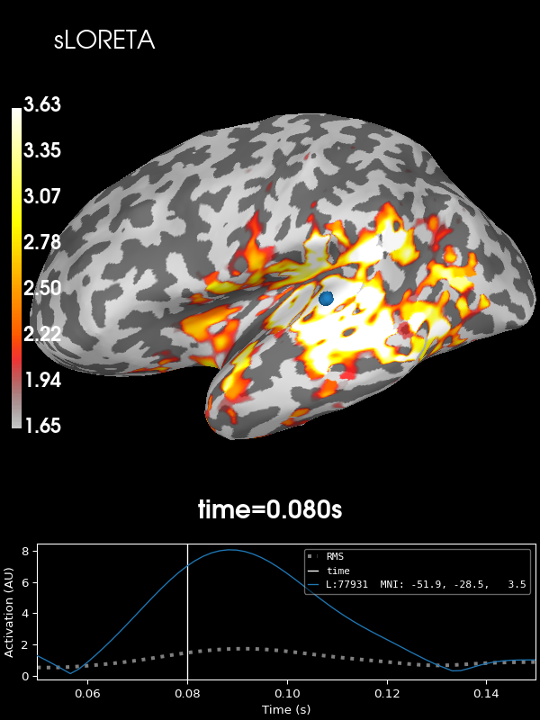
然后是 sLORETA:
stc = abs(apply_inverse(evoked, inv, lambda2, "sLORETA", verbose=True))
brain = stc.plot(**kwargs)
brain.add_text(0.1, 0.9, "sLORETA", "title", font_size=14)
Preparing the inverse operator for use...
    Scaled noise and source covariance from nave = 1 to nave = 61
    Created the regularized inverter
    Created an SSP operator (subspace dimension = 3)
    Created the whitener using a noise covariance matrix with rank 302 (3 small eigenvalues omitted)
    Computing noise-normalization factors (sLORETA)...
[done]
Applying inverse operator to "Right Auditory"...
    Picked 305 channels from the data
    Computing inverse...
    Eigenleads need to be weighted ...
    Computing residual...
    Explained  78.4% variance
    sLORETA...
[done]
Using control points [1.65359441 2.22223216 3.63030546]
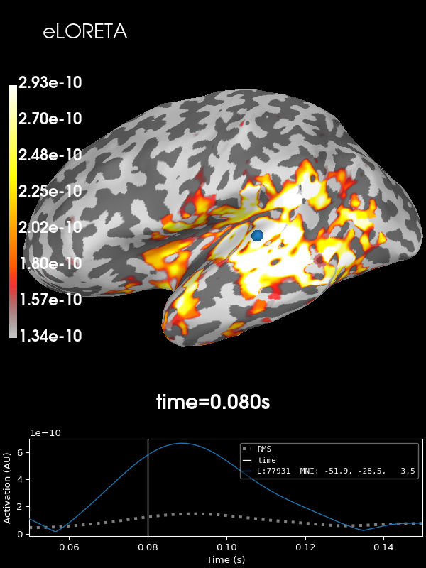
最后是 eLORETA:
stc = abs(apply_inverse(evoked, inv, lambda2, "eLORETA", verbose=True))
brain = stc.plot(**kwargs)
brain.add_text(0.1, 0.9, "eLORETA", "title", font_size=14)
del inv
Preparing the inverse operator for use...
    Scaled noise and source covariance from nave = 1 to nave = 61
    Created the regularized inverter
    Created an SSP operator (subspace dimension = 3)
    Created the whitener using a noise covariance matrix with rank 302 (3 small eigenvalues omitted)
    Computing optimized source covariance (eLORETA)...
        Fitting up to 20 iterations...
        Converged on iteration 11 (7.1e-07 < 1e-06)
        Updating inverse with weighted eigen leads
[done]
Applying inverse operator to "Right Auditory"...
    Picked 305 channels from the data
    Computing inverse...
    Eigenleads already weighted ...
    Computing residual...
    Explained  78.0% variance
[done]
Using control points [1.34003429e-10 1.79067976e-10 2.93243713e-10]
自由朝向#
现在我们完全不约束偶极子的朝向,创建一个自由朝向的逆算子。
inv = make_inverse_operator(evoked.info, fwd, cov, loose=1.0, depth=0.8, verbose=True)
del fwd
Computing inverse operator with 305 channels.
    305 out of 306 channels remain after picking
Selected 305 channels
Creating the depth weighting matrix...
    203 planar channels
    limit = 7265/7498 = 10.037797
    scale = 2.52065e-08 exp = 0.8
Whitening the forward solution.
    Created an SSP operator (subspace dimension = 3)
Computing rank from covariance with rank=None
    Using tolerance 3.3e-13 (2.2e-16 eps * 305 dim * 4.8  max singular value)
    Estimated rank (mag + grad): 302
    MEG: rank 302 computed from 305 data channels with 3 projectors
    Setting small MEG eigenvalues to zero (without PCA)
Creating the source covariance matrix
Adjusting source covariance matrix.
Computing SVD of whitened and weighted lead field matrix.
    largest singular value = 4.61893
    scaling factor to adjust the trace = 1.8713e+19 (nchan = 305 nzero = 3)
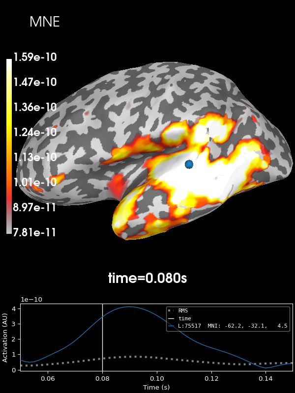
让我们用 MNE 查看当前估计。为简化可视化,我们将取源估计的绝对值。
stc = apply_inverse(evoked, inv, lambda2, "MNE", verbose=True)
brain = stc.plot(**kwargs)
brain.add_text(0.1, 0.9, "MNE", "title", font_size=14)
Preparing the inverse operator for use...
    Scaled noise and source covariance from nave = 1 to nave = 61
    Created the regularized inverter
    Created an SSP operator (subspace dimension = 3)
    Created the whitener using a noise covariance matrix with rank 302 (3 small eigenvalues omitted)
Applying inverse operator to "Right Auditory"...
    Picked 305 channels from the data
    Computing inverse...
    Eigenleads need to be weighted ...
    Computing residual...
    Explained  78.5% variance
    Combining the current components...
[done]
Using control points [7.81398590e-11 1.00293217e-10 1.59049573e-10]
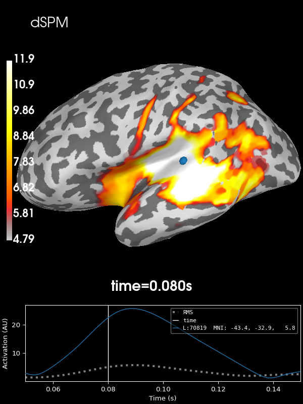
接下来使用默认的噪声归一化方法 dSPM:
stc = apply_inverse(evoked, inv, lambda2, "dSPM", verbose=True)
brain = stc.plot(**kwargs)
brain.add_text(0.1, 0.9, "dSPM", "title", font_size=14)
Preparing the inverse operator for use...
    Scaled noise and source covariance from nave = 1 to nave = 61
    Created the regularized inverter
    Created an SSP operator (subspace dimension = 3)
    Created the whitener using a noise covariance matrix with rank 302 (3 small eigenvalues omitted)
    Computing noise-normalization factors (dSPM)...
[done]
Applying inverse operator to "Right Auditory"...
    Picked 305 channels from the data
    Computing inverse...
    Eigenleads need to be weighted ...
    Computing residual...
    Explained  78.5% variance
    Combining the current components...
    dSPM...
[done]
Using control points [ 4.79225614  6.45181115 11.88420759]
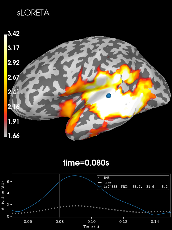
sLORETA:
stc = apply_inverse(evoked, inv, lambda2, "sLORETA", verbose=True)
brain = stc.plot(**kwargs)
brain.add_text(0.1, 0.9, "sLORETA", "title", font_size=14)
Preparing the inverse operator for use...
    Scaled noise and source covariance from nave = 1 to nave = 61
    Created the regularized inverter
    Created an SSP operator (subspace dimension = 3)
    Created the whitener using a noise covariance matrix with rank 302 (3 small eigenvalues omitted)
    Computing noise-normalization factors (sLORETA)...
[done]
Applying inverse operator to "Right Auditory"...
    Picked 305 channels from the data
    Computing inverse...
    Eigenleads need to be weighted ...
    Computing residual...
    Explained  78.5% variance
    Combining the current components...
    sLORETA...
[done]
Using control points [1.65906465 2.11446799 3.4224023 ]
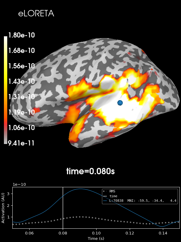
最后是 eLORETA:
stc = apply_inverse(
    evoked, inv, lambda2, "eLORETA", verbose=True, method_params=dict(eps=1e-4)
)  # larger eps just for speed
brain = stc.plot(**kwargs)
brain.add_text(0.1, 0.9, "eLORETA", "title", font_size=14)
Preparing the inverse operator for use...
    Scaled noise and source covariance from nave = 1 to nave = 61
    Created the regularized inverter
    Created an SSP operator (subspace dimension = 3)
    Created the whitener using a noise covariance matrix with rank 302 (3 small eigenvalues omitted)
    Computing optimized source covariance (eLORETA)...
        Using independent orientation weights
        Fitting up to 20 iterations (this make take a while)...
        Converged on iteration 7 (6.7e-05 < 0.0001)
        Updating inverse with weighted eigen leads
[done]
Applying inverse operator to "Right Auditory"...
    Picked 305 channels from the data
    Computing inverse...
    Eigenleads already weighted ...
    Computing residual...
    Explained  78.2% variance
    Combining the current components...
[done]
Using control points [9.41240750e-11 1.15338772e-10 1.80101709e-10]
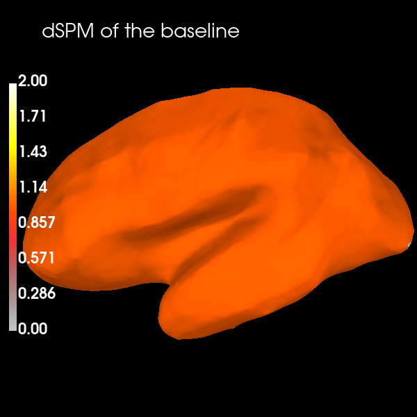
还有一个值得注意的有趣性质:通过可视化用于计算逆算子的噪声协方差的源重建结果,可以很容易地看出 dSPM 的噪声归一化效果——它在整个大脑上都取值为 1(在此处的色图中显示为橙色):
stc_baseline = apply_inverse_cov(
    cov, evoked.info, inv, lambda2=lambda2, method="dSPM", verbose=True
)
kwargs_baseline = kwargs.copy()
kwargs_baseline["clim"] = dict(kind="value", lims=[0, 1, 2])
brain = stc_baseline.plot(**kwargs_baseline)
brain.add_text(0.1, 0.9, "dSPM of the baseline", "title", font_size=14)
Preparing the inverse operator for use...
    Scaled noise and source covariance from nave = 1 to nave = 1
    Created the regularized inverter
    Created an SSP operator (subspace dimension = 3)
    Created the whitener using a noise covariance matrix with rank 302 (3 small eigenvalues omitted)
    Computing noise-normalization factors (dSPM)...
[done]
Applying inverse operator to "cov"...
    Picked 305 channels from the data
    Computing inverse...
    Eigenleads need to be weighted ...
    Computing residual...
    Explained  45.3% variance
    dSPM...
    Combining the current components...
[done]
脚本总运行时间:(0 分钟 21.140 秒)