
注意
转到末尾下载完整示例代码。
设置 EEG 参考#
本教程介绍如何在 MNE-Python 中设置或更改 EEG 参考。
照例,我们先导入所需的模块、加载一些示例数据,并裁剪数据以节省内存。由于本教程专门讨论 EEG,我们还会将数据集限制为少数几个 EEG 通道,以便更清楚地查看绘图:
# Authors: The MNE-Python contributors.
# License: BSD-3-Clause
# Copyright the MNE-Python contributors.
import os

import mne

sample_data_folder = mne.datasets.sample.data_path()
sample_data_raw_file = os.path.join(
    sample_data_folder, "MEG", "sample", "sample_audvis_raw.fif"
)
raw = mne.io.read_raw_fif(sample_data_raw_file, verbose=False)
raw.crop(tmax=60).load_data()
raw.pick([f"EEG 0{n:02}" for n in range(41, 60)])
Reading 0 ... 36037 = 0.000 ... 60.000 secs...
背景#
EEG 测量的是每个电极与参考电极之间的电压(电位差)。这意味着参考电极上存在的任何信号都会被从所有测量电极中减去。因此,理想的参考信号应当不包含任何脑特异性的电位波动,同时又能捕获测量电极所拾取到的全部环境噪声/干扰。
在实践中,这意味着参考电极通常放置在受试者身体上靠近头部的位置(这样任何环境干扰对参考电极和测量电极的影响相似),但又要尽可能远离神经源(这样参考信号不会拾取到源于大脑的波动)。典型的参考位置包括受试者的耳垂、鼻尖、乳突或锁骨。这些位置各有优缺点,一方面在于它们拾取多少脑信号(例如,与其他位置相比乳突会拾取相当多的脑信号),另一方面在于它们拾取多少环境噪声(例如,耳垂电极容易移位,且其信号与同侧头部电极更为相似)。
即使没有专门指定某个电极作为参考,EEG 记录硬件仍会将某个头皮电极视为参考,记录软件可能会也可能不会将其显示给你(它可能表现为完全平坦的通道,或者软件在显示前减去了所有信号的平均值,使其看起来像没有参考)。
设置或更改参考通道#
如果你想使用与原始数据记录和/或保存时不同的参考来重新计算数据,MNE-Python 在 Raw 对象上提供了 set_eeg_reference() 方法,以及 mne.add_reference_channels() 函数。要使用已有通道作为新参考,请使用 set_eeg_reference() 方法;你也可以指定多个已有电极作为参考通道,就像有时使用乳突参考那样:
# code lines below are commented out because the sample data doesn't have
# earlobe or mastoid channels, so this is just for demonstration purposes:

# use a single channel reference (left earlobe)
# raw.set_eeg_reference(ref_channels='A1')

# use average of mastoid channels as reference
# raw.set_eeg_reference(ref_channels=['M1', 'M2'])

# use a bipolar reference (contralateral)
# raw.set_bipolar_reference(anode='F3', cathode='F4')
如果某个头皮电极曾被用作参考,却没有与原始数据一起保存(参考通道通常不会被保存),你可能希望在重新参考前将其加回数据集。例如,如果你的 EEG 系统以通道 Fp1 作为参考进行记录,但数据文件中未包含 Fp1,那么使用 set_eeg_reference() 将(比如)Cz 设为新参考时,会减去 Cz 处的信号,却无法恢复 Fp1 处的信号。在这种情况下,可以在重新参考之前使用 add_reference_channels() 将 Fp1 作为平坦通道加回。(由于我们的示例数据不使用 10-20 电极命名系统,下面的示例将 EEG 999 作为缺失的参考加入,然后将参考设置为 EEG 050。)以下是数据在原始状态下的样子:
raw.plot()
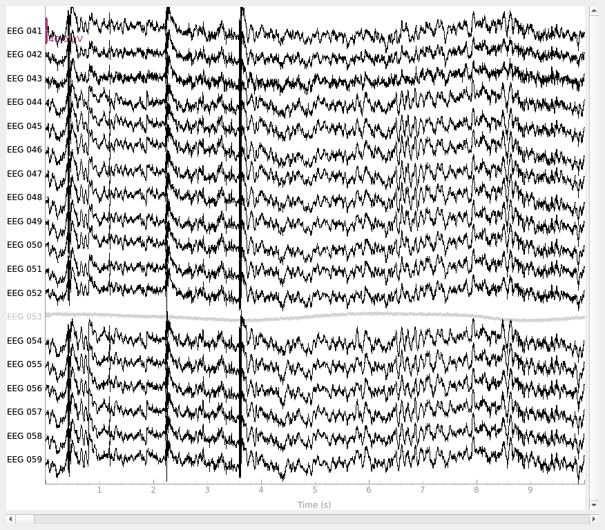
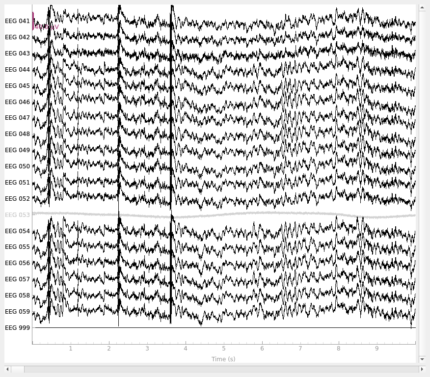
默认情况下,add_reference_channels() 返回一个副本,因此我们稍后仍可回到原始的 raw 对象。如果希望就地修改现有的 Raw 对象,可以指定 copy=False。
# add new reference channel (all zero)
raw_new_ref = mne.add_reference_channels(raw, ref_channels="EEG 999")
raw_new_ref.plot()
# set reference to `EEG 050`
raw_new_ref.set_eeg_reference(ref_channels="EEG 050")
raw_new_ref.plot()
EEG channel type selected for re-referencing
Applying a custom ('EEG',) reference.
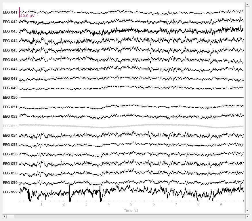
请注意,新参考(EEG 050)现在已是平坦的,而我们加回数据的原始参考通道(EEG 999)具有非零信号。还需注意,EEG 053(在 raw.info['bads'] 中标记为“坏”)不受重新参考的影响。
设置平均参考#
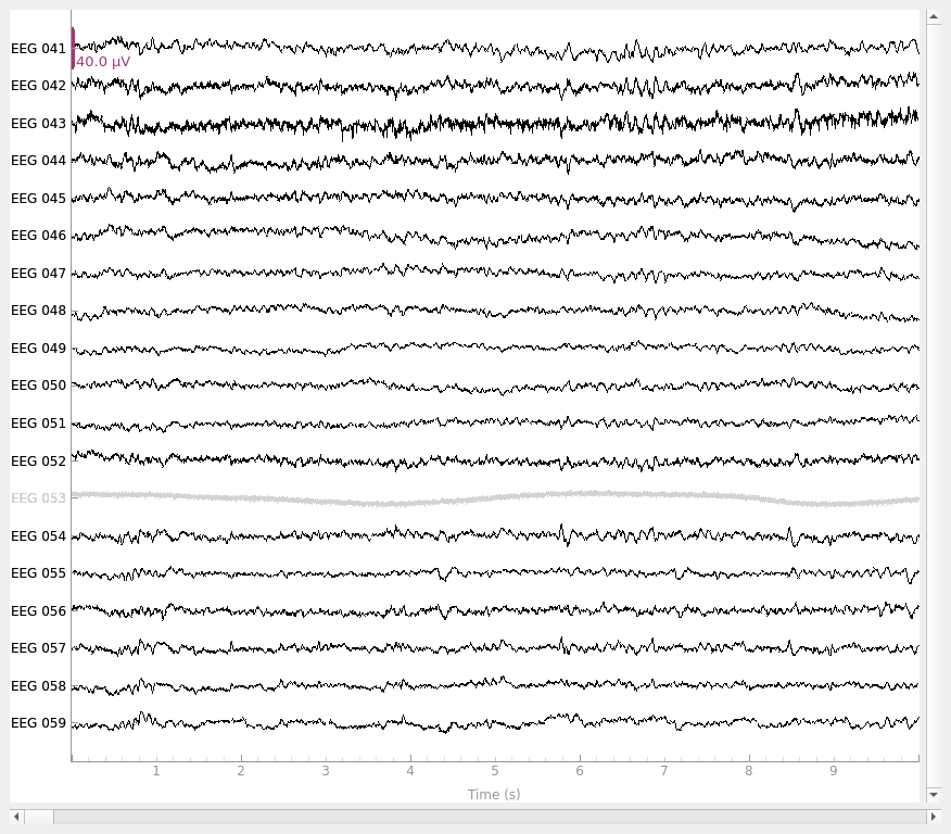
要设置取所有通道平均值的“虚拟参考”,可以使用 set_eeg_reference() 并指定 ref_channels='average'。与上面一样,这不会影响任何标记为“坏”的通道,计算平均值时也不会包含坏通道。不过它会就地修改 Raw 对象,因此我们先制作一个副本,以便稍后仍能回到未修改的 Raw 对象:
# use the average of all channels as reference
raw_avg_ref = raw.copy().set_eeg_reference(ref_channels="average")
raw_avg_ref.plot()
EEG channel type selected for re-referencing
Applying average reference.
Applying a custom ('EEG',) reference.
注意
在传感器空间分析中执行平均参考时,原始参考电极应作为零填充通道存在。如果不存在,必须先使用 add_reference_channels() 将其添加,然后再调用 set_eeg_reference()。这是避免对参考产生偏倚所必需的 [1],否则被减去的参考信号会除以 n_channels,而不是正确的 n_channels + 1(即包含原始参考通道)。
将平均参考创建为投影算子#
如果使用平均参考,可以通过指定 projection=True 将参考创建为投影算子,而不是立即从数据中减去参考:
raw.set_eeg_reference("average", projection=True)
print(raw.info["projs"])
EEG channel type selected for re-referencing
Adding average EEG reference projection.
1 projection items deactivated
Average reference projection was added, but has not been applied yet. Use the apply_proj method to apply it.
[<Projection | Average EEG reference, active : False, n_channels : 18>]
将平均参考创建为投影算子有几个优点:
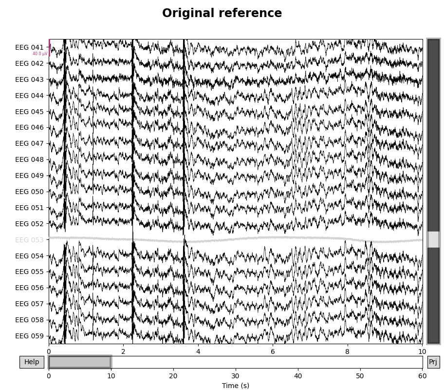
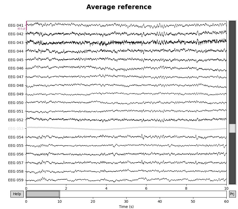
绘图时可以打开或关闭投影算子,因此很容易直观地查看平均参考对数据的影响。
如果后续有更多通道被标记为“坏”,或者之后选择了通道子集,投影算子会重新计算以考虑这些变化(从而保证信号均值为零)。
如果还有其他未应用的投影算子影响 EEG 通道(例如用于去除心跳或眨眼伪迹的 SSP 投影算子),则在这些投影算子被应用或移除之前无法执行 EEG 重新参考;而将 EEG 参考添加为投影算子则不受此限制。(我们上面将非投影算子形式的平均参考应用于
raw_avg_ref时之所以没有出现这个问题,是因为示例数据.fif文件中包含的空房间投影算子仅针对磁强计计算。)
for title, proj in zip(["Original", "Average"], [False, True]):
    with mne.viz.use_browser_backend("matplotlib"):
        fig = raw.plot(proj=proj, n_channels=len(raw))
    # make room for title
    fig.subplots_adjust(top=0.9)
    fig.suptitle(f"{title} reference", size="xx-large", weight="bold")
Using matplotlib as 2D backend.
Using qt as 2D backend.
Using matplotlib as 2D backend.
Using qt as 2D backend.
使用无穷远参考(REST)#
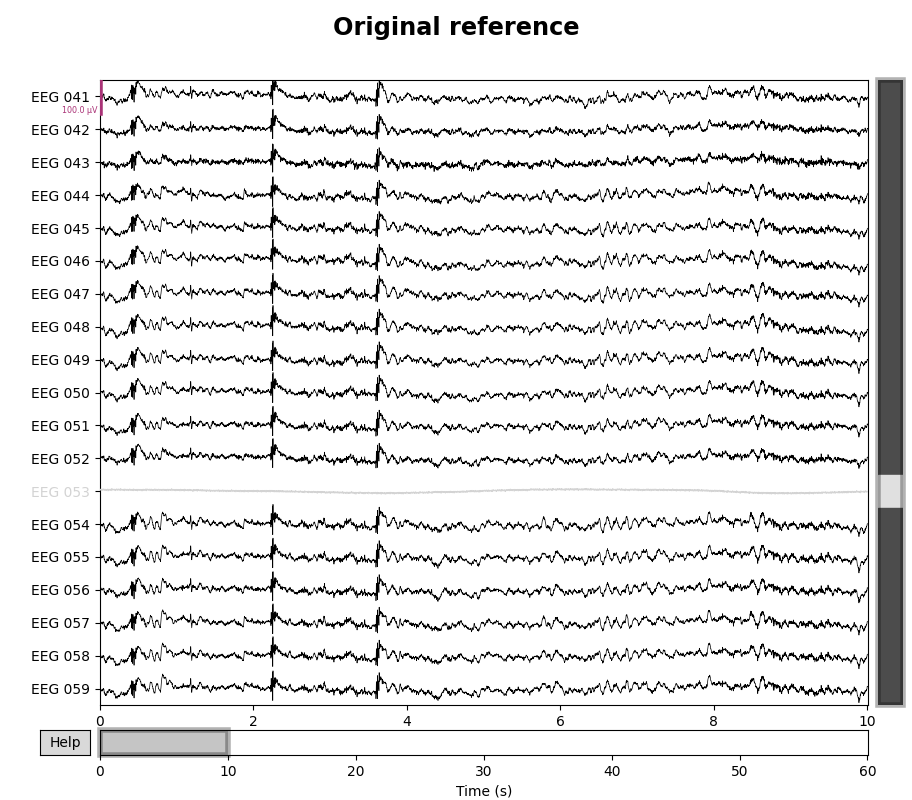
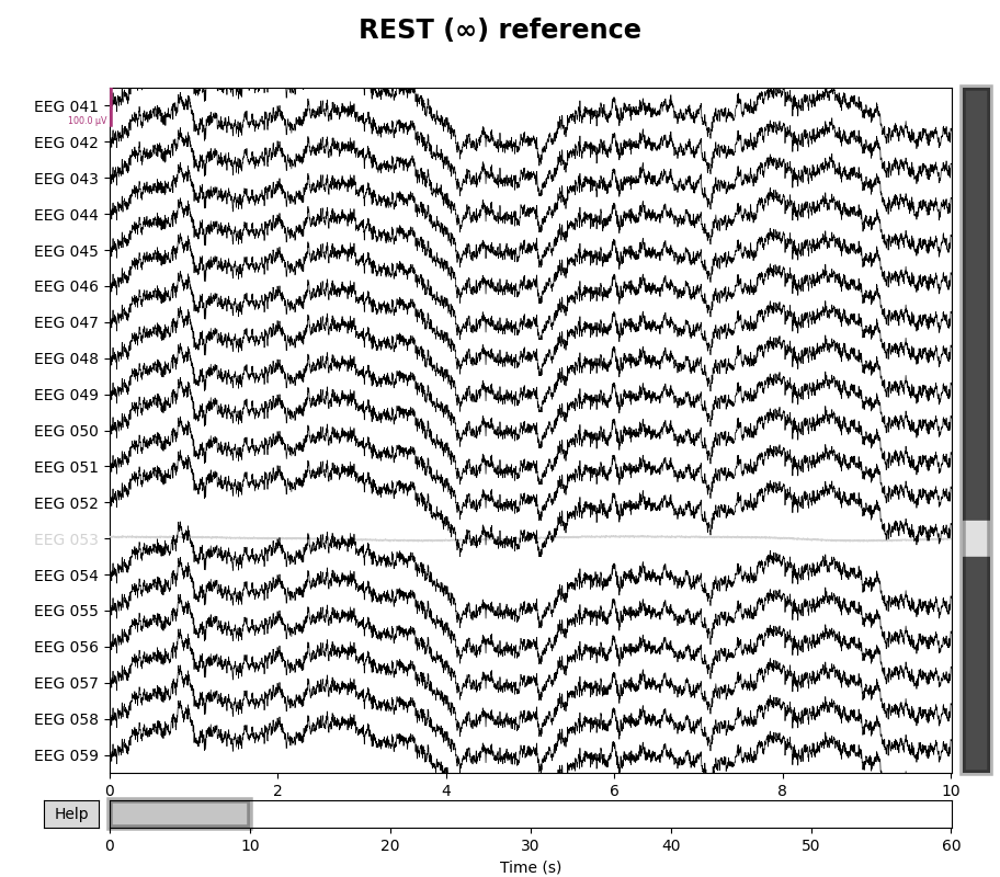
使用 [2] 中描述的“无穷远点”参考技术需要一个前向模型,我们可以通过几个步骤创建它。这里我们使用较大的顶点间距(pos=15 mm)以减少计算时间;在实际数据分析中,5 mm 的间距更为常见:
raw.del_proj()  # remove our average reference projector first
sphere = mne.make_sphere_model("auto", "auto", raw.info)
src = mne.setup_volume_source_space(sphere=sphere, exclude=30.0, pos=15.0)
forward = mne.make_forward_solution(raw.info, trans=None, src=src, bem=sphere)
raw_rest = raw.copy().set_eeg_reference("REST", forward=forward)

for title, _raw in zip(["Original", "REST (∞)"], [raw, raw_rest]):
    with mne.viz.use_browser_backend("matplotlib"):
        fig = _raw.plot(n_channels=len(raw), scalings=dict(eeg=5e-5))
    # make room for title
    fig.subplots_adjust(top=0.9)
    fig.suptitle(f"{title} reference", size="xx-large", weight="bold")
Fitted sphere radius:         91.2 mm
Origin head coordinates:      -4.2 16.4 51.8 mm
Origin device coordinates:    1.5 18.2 -10.1 mm

Equiv. model fitting -> RV = 0.00347813 %%
mu1 = 0.944815    lambda1 = 0.13694
mu2 = 0.667658    lambda2 = 0.683728
mu3 = -0.286487    lambda3 = -0.0102992
Set up EEG sphere model with scalp radius    91.2 mm

Sphere                : origin at (-4.2 16.4 51.8) mm
              radius  : 82.1 mm
grid                  : 15.0 mm
mindist               : 5.0 mm
Exclude               : 30.0 mm

Setting up the sphere...
Surface CM = (  -4.2   16.4   51.8) mm
Surface fits inside a sphere with radius   82.1 mm
Surface extent:
    x =  -86.2 ...   77.9 mm
    y =  -65.7 ...   98.4 mm
    z =  -30.2 ...  133.9 mm
Grid extent:
    x =  -90.0 ...   90.0 mm
    y =  -75.0 ...  105.0 mm
    z =  -45.0 ...  135.0 mm
2197 sources before omitting any.
654 sources after omitting infeasible sources not within 30.0 - 82.1 mm.
Source spaces are in MRI coordinates.
Checking that the sources are inside the surface and at least    5.0 mm away (will take a few...)
    117 source space point omitted because of the    5.0-mm distance limit.
537 sources remaining after excluding the sources outside the surface and less than    5.0 mm inside.
Adjusting the neighborhood info.
Source space : MRI voxel -> MRI (surface RAS)
    0.015000 0.000000 0.000000     -90.00 mm
    0.000000 0.015000 0.000000     -75.00 mm
    0.000000 0.000000 0.015000     -45.00 mm
    0.000000 0.000000 0.000000       1.00
Source space          : <SourceSpaces: [<discrete, n_used=537>] MRI (surface RAS) coords, ~559 KiB>
MRI -> head transform : identity
Measurement data      : instance of Info
Sphere model      : origin at [-0.00415196  0.01635826  0.05183149] mm
Standard field computations
Do computations in head coordinates
Free source orientations

Read 1 source spaces a total of 537 active source locations

Coordinate transformation: MRI (surface RAS) -> head
    1.000000 0.000000 0.000000       0.00 mm
    0.000000 1.000000 0.000000       0.00 mm
    0.000000 0.000000 1.000000       0.00 mm
    0.000000 0.000000 0.000000       1.00

Read  19 EEG channels from info
Head coordinate coil definitions created.
Source spaces are now in head coordinates.

Using the sphere model.

Source spaces are in head coordinates.
Checking that the sources are inside the surface (will take a few...)
Using the equivalent source approach in the homogeneous sphere for EEG
Computing EEG at 537 source locations (free orientations)...

Finished.
EEG channel type selected for re-referencing
Applying REST reference.
Applying a custom ('EEG',) reference.
    18 out of 19 channels remain after picking
Using matplotlib as 2D backend.
Using qt as 2D backend.
Using matplotlib as 2D backend.
Using qt as 2D backend.
使用双极参考#
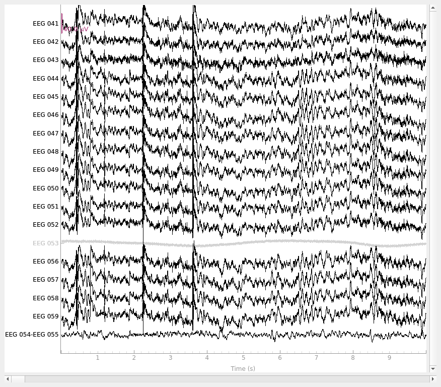
要创建双极参考,可以使用 set_bipolar_reference(),并分别指定阳极和阴极的通道名称;该函数会创建一个新的虚拟通道,取两个指定通道(阳极和阴极)之差,并默认删除原始通道。新虚拟通道将标注为阳极的通道信息,位置默认设置为 (0, 0, 0),线圈类型默认设置为 EEG_BIPOLAR。这里我们按照 [3] 所述,在通道 EEG 054 和 EEG 055 之间使用对侧/横向双极参考,从而创建一个名为 EEG 054-EEG 055 的新虚拟通道。
raw_bip_ref = mne.set_bipolar_reference(raw, anode="EEG 054", cathode="EEG 055")
raw_bip_ref.plot()
EEG channel type selected for re-referencing
Creating RawArray with float64 data, n_channels=1, n_times=36038
    Range : 25800 ... 61837 =     42.956 ...   102.956 secs
Ready.
Added the following bipolar channels:
EEG 054-EEG 055
EEG 参考与源建模#
如果你计划进行源建模(无论使用 EEG 还是 EEG/MEG 联合数据),强烈建议采用“平均参考作为投影”的方法。使用平均参考很重要,因为使用某个特定的参考传感器(甚至少数几个传感器的平均值)会将参考传感器的前向模型误差扩散到所有传感器,从而在计算源估计时实际上放大了参考传感器的重要性。相比之下,使用所有 EEG 通道的平均值作为参考会将前向建模误差均匀分布到各通道,因此在源估计过程中没有哪个通道会被赋予更大的权重。更多信息另请参阅 FieldTrip 关于平均参考的常见问题解答。
上一节已经提到将平均参考指定为投影算子的主要原因:平均参考投影算子在通道被剔除时会自适应调整,确保执行源建模时信号始终为零均值。相比之下,通过传统减法方法应用平均参考则没有这种保证。
重要
由于这些原因,在进行逆成像时,如果存在 EEG 通道,且指定的不是平均参考投影算子策略,MNE-Python 将引发 ValueError。为确保正确运行,请考虑调用 set_eeg_reference(projection=True) 将平均参考添加为投影算子。
参考文献#
脚本总运行时间:(0 分钟 6.653 秒)