
非官方中文翻译
本页译自 MNE-Python 官方文档:
查看英文原文 ↗。
文档版权归 MNE Developers 所有(BSD-3-Clause)。
说明
转到末尾下载完整示例代码。
使用类 XFit 多偶极子模型计算源时间过程#
MEGIN 的 XFit 程序提供“引导式 ECD 建模”界面,可交互拟合多个偶极子。通过手动选择传感器子集与时间范围,可把偶极子拟合到特定信号成分;随后用多偶极子模型计算源时间过程。相比逐个单独拟合,多偶极子模型的优势在于:当多个偶极子贡献同一信号成分时,模型能确保分配给一个偶极子的活动不会同时分配给另一个。本示例展示如何构建多偶极子模型,以估计诱发数据或单试次分段的源时间过程。
推荐使用 XFit 进行引导式 ECD 建模,因为它提供便捷的图形界面。随后可用 mne.read_dipole() 函数把偶极子导入 MNE-Python,构建并应用多偶极子模型。此外,本示例也演示仅用 MNE-Python 完成引导式 ECD 建模;它不如 XFit 方便,但具有可复现的优点。
# Author: Marijn van Vliet <w.m.vanvliet@gmail.com>
#
# License: BSD-3-Clause
# Copyright the MNE-Python contributors.
导入所有依赖,并设置 MNE-Sample 数据集的数据路径。
import matplotlib.pyplot as plt
import numpy as np

import mne
from mne.channels import read_vectorview_selection
from mne.datasets import sample
from mne.minimum_norm import apply_inverse, apply_inverse_epochs, make_inverse_operator

data_path = sample.data_path()
meg_path = data_path / "MEG" / "sample"
raw_fname = meg_path / "sample_audvis_raw.fif"
cov_fname = meg_path / "sample_audvis-shrunk-cov.fif"
bem_dir = data_path / "subjects" / "sample" / "bem"
bem_fname = bem_dir / "sample-5120-5120-5120-bem-sol.fif"
trans_fname = meg_path / "sample_audvis_raw-trans.fif"
读取 audvis 实验的 MEG 数据,为左侧与右侧听觉条件创建分段与诱发数据。
raw = mne.io.read_raw_fif(raw_fname)
raw = raw.pick(picks=["meg", "eog", "stim"])
info = raw.info

# Create epochs for auditory events
events = mne.find_events(raw)
event_id = dict(right=1, left=2)
epochs = mne.Epochs(
    raw,
    events,
    event_id,
    tmin=-0.1,
    tmax=0.3,
    baseline=(None, 0),
    reject=dict(mag=4e-12, grad=4000e-13, eog=150e-6),
)

# Create evokeds for left and right auditory stimulation
evoked_left = epochs["left"].average()
evoked_right = epochs["right"].average()
Opening raw data file /home/circleci/mne_data/MNE-sample-data/MEG/sample/sample_audvis_raw.fif...
    Read a total of 3 projection items:
        PCA-v1 (1 x 10²)  idle
        PCA-v2 (1 x 10²)  idle
        PCA-v3 (1 x 10²)  idle
    Range : 25800 ... 192599 =     42.956 ...   320.670 secs
Ready.
Finding events on: STI 014
320 events found on stim channel STI 014
Event IDs: [ 1  2  3  4  5 32]
Not setting metadata
145 matching events found
Setting baseline interval to [-0.09989760657919393, 0.0] s
Applying baseline correction (mode: mean)
Created an SSP operator (subspace dimension = 3)
3 projection items activated
    Rejecting  epoch based on EOG : ['EOG 061']
    Rejecting  epoch based on EOG : ['EOG 061']
    Rejecting  epoch based on EOG : ['EOG 061']
    Rejecting  epoch based on EOG : ['EOG 061']
    Rejecting  epoch based on EOG : ['EOG 061']
    Rejecting  epoch based on EOG : ['EOG 061']
    Rejecting  epoch based on EOG : ['EOG 061']
    Rejecting  epoch based on EOG : ['EOG 061']
    Rejecting  epoch based on EOG : ['EOG 061']
    Rejecting  epoch based on MAG : ['MEG 1711']
    Rejecting  epoch based on EOG : ['EOG 061']
    Rejecting  epoch based on EOG : ['EOG 061']
    Rejecting  epoch based on EOG : ['EOG 061']
    Rejecting  epoch based on EOG : ['EOG 061']
引导式偶极子建模——在手动选择的时间窗内对手动选择的传感器子集拟合偶极子——现在可在 MEGIN 的 XFit 中对上面计算的诱发数据执行;不过也可以完全在 MNE-Python 中完成。
# Setup conductor model
cov = mne.read_cov(cov_fname)  # bad channels were already excluded here
bem = mne.read_bem_solution(bem_fname)

# Fit two dipoles at t=80ms. The first dipole is fitted using only the sensors
# on the left side of the helmet. The second dipole is fitted using only the
# sensors on the right side of the helmet.
picks_left = read_vectorview_selection("Left", info=info)
evoked_fit_left = evoked_left.copy().crop(0.08, 0.08)
evoked_fit_left.pick(picks_left)
cov_fit_left = cov.copy().pick_channels(picks_left, ordered=True)

picks_right = read_vectorview_selection("Right", info=info)
picks_right = list(set(picks_right) - set(info["bads"]))
evoked_fit_right = evoked_right.copy().crop(0.08, 0.08)
evoked_fit_right.pick(picks_right)
cov_fit_right = cov.copy().pick_channels(picks_right, ordered=True)

# Any SSS projections that are active on this data need to be re-normalized
# after picking channels.
evoked_fit_left.info.normalize_proj()
evoked_fit_right.info.normalize_proj()
cov_fit_left["projs"] = evoked_fit_left.info["projs"]
cov_fit_right["projs"] = evoked_fit_right.info["projs"]

# Fit the dipoles with the subset of sensors.
kwargs = dict(bem=bem, trans=trans_fname)
dip_left, _ = mne.fit_dipole(evoked_fit_left, cov_fit_left, **kwargs)
dip_right, _ = mne.fit_dipole(evoked_fit_right, cov_fit_right, **kwargs)
    365 x 365 full covariance (kind = 1) found.
    Read a total of 4 projection items:
        PCA-v1 (1 x 10²) active
        PCA-v2 (1 x 10²) active
        PCA-v3 (1 x 10²) active
        Average EEG reference (1 x 59) active
Loading surfaces...

Loading the solution matrix...

Three-layer model surfaces loaded.
Loaded linear collocation BEM solution from /home/circleci/mne_data/MNE-sample-data/subjects/sample/bem/sample-5120-5120-5120-bem-sol.fif
BEM               : <ConductorModel | BEM (3 layers) solver=mne>
MRI transform     : /home/circleci/mne_data/MNE-sample-data/MEG/sample/sample_audvis_raw-trans.fif
Head origin       :   -4.2   19.3   65.3 mm rad =   72.3 mm.
Guess grid        :   20.0 mm
Guess mindist     :    5.0 mm
Guess exclude     :   20.0 mm
Using normal MEG coil definitions.
Noise covariance  : <Covariance | kind : full, shape : (153, 153), range : [-1.4e-23, +3.7e-23], n_samples : 38720>

Coordinate transformation: MRI (surface RAS) -> head
    0.999310 0.009985 -0.035787      -3.17 mm
    0.012759 0.812405 0.582954       6.86 mm
    0.034894 -0.583008 0.811716      28.88 mm
    0.000000 0.000000 0.000000       1.00
Coordinate transformation: MEG device -> head
    0.991420 -0.039936 -0.124467      -6.13 mm
    0.060661 0.984012 0.167456       0.06 mm
    0.115790 -0.173570 0.977991      64.74 mm
    0.000000 0.000000 0.000000       1.00
0 bad channels total
Read 153 MEG channels from info
105 coil definitions read
Coordinate transformation: MEG device -> head
    0.991420 -0.039936 -0.124467      -6.13 mm
    0.060661 0.984012 0.167456       0.06 mm
    0.115790 -0.173570 0.977991      64.74 mm
    0.000000 0.000000 0.000000       1.00
MEG coil definitions created in head coordinates.
Decomposing the sensor noise covariance matrix...
    Created an SSP operator (subspace dimension = 3)
Computing rank from covariance with rank=None
    Using tolerance 1.1e-13 (2.2e-16 eps * 153 dim * 3.2  max singular value)
    Estimated rank (mag + grad): 150
    MEG: rank 150 computed from 153 data channels with 3 projectors
    Setting small MEG eigenvalues to zero (without PCA)
    Created the whitener using a noise covariance matrix with rank 150 (3 small eigenvalues omitted)

---- Computing the forward solution for the guesses...
Guess surface (inner skull) is in MRI (surface RAS) coordinates
Filtering (grid =     20 mm)...
Surface CM = (   0.7  -10.0   44.3) mm
Surface fits inside a sphere with radius   91.8 mm
Surface extent:
    x =  -66.7 ...   68.8 mm
    y =  -88.0 ...   79.0 mm
    z =  -44.5 ...  105.8 mm
Grid extent:
    x =  -80.0 ...   80.0 mm
    y = -100.0 ...   80.0 mm
    z =  -60.0 ...  120.0 mm
900 sources before omitting any.
396 sources after omitting infeasible sources not within 20.0 - 91.8 mm.
Source spaces are in MRI coordinates.
Checking that the sources are inside the surface and at least    5.0 mm away (will take a few...)
Checking surface interior status for 396 points...
    Found  42/396 points inside  an interior sphere of radius   43.6 mm
    Found   0/396 points outside an exterior sphere of radius   91.8 mm
    Found 186/354 points outside using surface Qhull
    Found   9/168 points outside using solid angles
    Total 201/396 points inside the surface
Interior check completed in 15.1 ms
    195 source space points omitted because they are outside the inner skull surface.
    45 source space points omitted because of the    5.0-mm distance limit.
156 sources remaining after excluding the sources outside the surface and less than    5.0 mm inside.
Go through all guess source locations...
[done 156 sources]
---- Fitted :    79.9 ms, distance to inner skull : 11.2567 mm
Projections have already been applied. Setting proj attribute to True.
1 time points fitted
BEM               : <ConductorModel | BEM (3 layers) solver=mne>
MRI transform     : /home/circleci/mne_data/MNE-sample-data/MEG/sample/sample_audvis_raw-trans.fif
Head origin       :   -4.2   19.3   65.3 mm rad =   72.3 mm.
Guess grid        :   20.0 mm
Guess mindist     :    5.0 mm
Guess exclude     :   20.0 mm
Using normal MEG coil definitions.
Noise covariance  : <Covariance | kind : full, shape : (152, 152), range : [-1.7e-23, +5.2e-23], n_samples : 38720>

Coordinate transformation: MRI (surface RAS) -> head
    0.999310 0.009985 -0.035787      -3.17 mm
    0.012759 0.812405 0.582954       6.86 mm
    0.034894 -0.583008 0.811716      28.88 mm
    0.000000 0.000000 0.000000       1.00
Coordinate transformation: MEG device -> head
    0.991420 -0.039936 -0.124467      -6.13 mm
    0.060661 0.984012 0.167456       0.06 mm
    0.115790 -0.173570 0.977991      64.74 mm
    0.000000 0.000000 0.000000       1.00
0 bad channels total
Read 152 MEG channels from info
105 coil definitions read
Coordinate transformation: MEG device -> head
    0.991420 -0.039936 -0.124467      -6.13 mm
    0.060661 0.984012 0.167456       0.06 mm
    0.115790 -0.173570 0.977991      64.74 mm
    0.000000 0.000000 0.000000       1.00
MEG coil definitions created in head coordinates.
Decomposing the sensor noise covariance matrix...
    Created an SSP operator (subspace dimension = 3)
Computing rank from covariance with rank=None
    Using tolerance 1.3e-13 (2.2e-16 eps * 152 dim * 3.8  max singular value)
    Estimated rank (mag + grad): 149
    MEG: rank 149 computed from 152 data channels with 3 projectors
    Setting small MEG eigenvalues to zero (without PCA)
    Created the whitener using a noise covariance matrix with rank 149 (3 small eigenvalues omitted)

---- Computing the forward solution for the guesses...
Guess surface (inner skull) is in MRI (surface RAS) coordinates
Filtering (grid =     20 mm)...
Surface CM = (   0.7  -10.0   44.3) mm
Surface fits inside a sphere with radius   91.8 mm
Surface extent:
    x =  -66.7 ...   68.8 mm
    y =  -88.0 ...   79.0 mm
    z =  -44.5 ...  105.8 mm
Grid extent:
    x =  -80.0 ...   80.0 mm
    y = -100.0 ...   80.0 mm
    z =  -60.0 ...  120.0 mm
900 sources before omitting any.
396 sources after omitting infeasible sources not within 20.0 - 91.8 mm.
Source spaces are in MRI coordinates.
Checking that the sources are inside the surface and at least    5.0 mm away (will take a few...)
Checking surface interior status for 396 points...
    Found  42/396 points inside  an interior sphere of radius   43.6 mm
    Found   0/396 points outside an exterior sphere of radius   91.8 mm
    Found 186/354 points outside using surface Qhull
    Found   9/168 points outside using solid angles
    Total 201/396 points inside the surface
Interior check completed in 11.9 ms
    195 source space points omitted because they are outside the inner skull surface.
    45 source space points omitted because of the    5.0-mm distance limit.
156 sources remaining after excluding the sources outside the surface and less than    5.0 mm inside.
Go through all guess source locations...
[done 156 sources]
---- Fitted :    79.9 ms, distance to inner skull : 12.3554 mm
Projections have already been applied. Setting proj attribute to True.
1 time points fitted
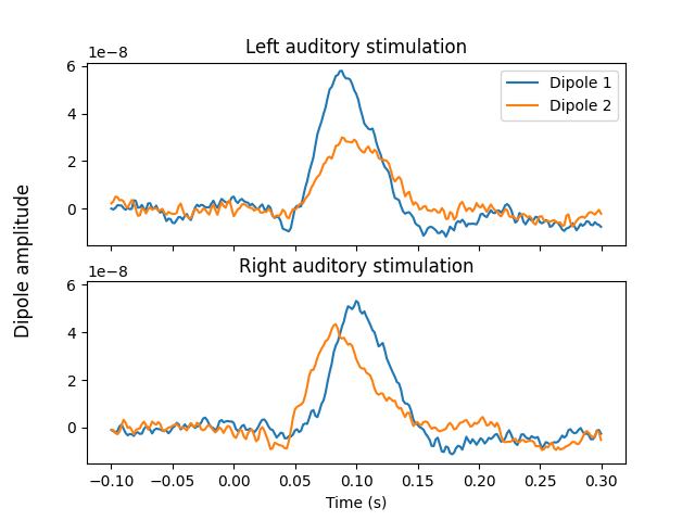
现在已得到偶极子的位置与朝向,使用 MNE 计算完整时间过程:同时为两个偶极子分配活动,同时防止二者之间的泄漏。我们使用很小的 lambda 值,确保两个偶极子都被充分利用。
fwd, _ = mne.make_forward_dipole([dip_left, dip_right], bem, info)

# Apply MNE inverse
inv = make_inverse_operator(info, fwd, cov, fixed=True, depth=0)
stc_left = apply_inverse(evoked_left, inv, method="MNE", lambda2=1e-6)
stc_right = apply_inverse(evoked_right, inv, method="MNE", lambda2=1e-6)

# Plot the timecourses of the resulting source estimate
fig, axes = plt.subplots(nrows=2, sharex=True, sharey=True)
axes[0].plot(stc_left.times, stc_left.data.T)
axes[0].set_title("Left auditory stimulation")
axes[0].legend(["Dipole 1", "Dipole 2"])
axes[1].plot(stc_right.times, stc_right.data.T)
axes[1].set_title("Right auditory stimulation")
axes[1].set_xlabel("Time (s)")
fig.supylabel("Dipole amplitude")
Positions (in meters) and orientations
2 sources
Source space          : <SourceSpaces: [<discrete, n_used=2>] head coords, ~2 KiB>
MRI -> head transform : identity
Measurement data      : instance of Info
Conductor model   : instance of ConductorModel
Accurate field computations
Do computations in head coordinates
Free source orientations

Read 1 source spaces a total of 2 active source locations

Coordinate transformation: MRI (surface RAS) -> head
    1.000000 0.000000 0.000000       0.00 mm
    0.000000 1.000000 0.000000       0.00 mm
    0.000000 0.000000 1.000000       0.00 mm
    0.000000 0.000000 0.000000       1.00

Read 306 MEG channels from info
105 coil definitions read
Coordinate transformation: MEG device -> head
    0.991420 -0.039936 -0.124467      -6.13 mm
    0.060661 0.984012 0.167456       0.06 mm
    0.115790 -0.173570 0.977991      64.74 mm
    0.000000 0.000000 0.000000       1.00
MEG coil definitions created in head coordinates.
Source spaces are now in head coordinates.

Employing the head->MRI coordinate transform with the BEM model.
BEM model instance of ConductorModel is now set up


Source spaces are in head coordinates.
Checking that the sources are inside the surface (will take a few...)
Checking surface interior status for 2 points...
    Found 0/2 points inside  an interior sphere of radius   43.6 mm
    Found 0/2 points outside an exterior sphere of radius   91.8 mm
    Found 0/2 points outside using surface Qhull
    Found 0/2 points outside using solid angles
    Total 2/2 points inside the surface
Interior check completed in 0.6 ms
Checking surface interior status for 306 points...
    Found   0/306 points inside  an interior sphere of radius   79.1 mm
    Found   0/306 points outside an exterior sphere of radius  161.3 mm
    Found 306/306 points outside using surface Qhull
    Found   0/  0 points outside using solid angles
    Total 0/306 points inside the surface
Interior check completed in 0.4 ms

Composing the field computation matrix...
Computing MEG at 2 source locations (free orientations)...

Finished.
    Changing to fixed-orientation forward solution with surface-based source orientations...
    [done]
Computing inverse operator with 305 channels.
    305 out of 306 channels remain after picking
Selected 305 channels
Whitening the forward solution.
    Created an SSP operator (subspace dimension = 3)
Computing rank from covariance with rank=None
    Using tolerance 3.5e-13 (2.2e-16 eps * 305 dim * 5.2  max singular value)
    Estimated rank (mag + grad): 302
    MEG: rank 302 computed from 305 data channels with 3 projectors
    Setting small MEG eigenvalues to zero (without PCA)
Creating the source covariance matrix
Adjusting source covariance matrix.
Computing SVD of whitened and weighted lead field matrix.
    largest singular value = 13.8846
    scaling factor to adjust the trace = 2.17572e+16 (nchan = 305 nzero = 3)
Preparing the inverse operator for use...
    Scaled noise and source covariance from nave = 1 to nave = 65
    Created the regularized inverter
    Created an SSP operator (subspace dimension = 3)
    Created the whitener using a noise covariance matrix with rank 302 (3 small eigenvalues omitted)
Applying inverse operator to "left"...
    Picked 305 channels from the data
    Computing inverse...
    Eigenleads need to be weighted ...
    Computing residual...
    Explained  13.9% variance
[done]
Preparing the inverse operator for use...
    Scaled noise and source covariance from nave = 1 to nave = 66
    Created the regularized inverter
    Created an SSP operator (subspace dimension = 3)
    Created the whitener using a noise covariance matrix with rank 302 (3 small eigenvalues omitted)
Applying inverse operator to "right"...
    Picked 305 channels from the data
    Computing inverse...
    Eigenleads need to be weighted ...
    Computing residual...
    Explained  15.3% variance
[done]
也可以对单试次分段拟合时间过程,这里对每个实验条件分别进行。
stcs_left = apply_inverse_epochs(epochs["left"], inv, lambda2=1e-6, method="MNE")
stcs_right = apply_inverse_epochs(epochs["right"], inv, lambda2=1e-6, method="MNE")
Preparing the inverse operator for use...
    Scaled noise and source covariance from nave = 1 to nave = 1
    Created the regularized inverter
    Created an SSP operator (subspace dimension = 3)
    Created the whitener using a noise covariance matrix with rank 302 (3 small eigenvalues omitted)
Picked 305 channels from the data
Computing inverse...
    Eigenleads need to be weighted ...
    Rejecting  epoch based on EOG : ['EOG 061']
Processing epoch : 1 / 73 (at most)
Processing epoch : 2 / 73 (at most)
Processing epoch : 3 / 73 (at most)
    Rejecting  epoch based on EOG : ['EOG 061']
Processing epoch : 4 / 73 (at most)
Processing epoch : 5 / 73 (at most)
Processing epoch : 6 / 73 (at most)
Processing epoch : 7 / 73 (at most)
Processing epoch : 8 / 73 (at most)
Processing epoch : 9 / 73 (at most)
Processing epoch : 10 / 73 (at most)
Processing epoch : 11 / 73 (at most)
Processing epoch : 12 / 73 (at most)
Processing epoch : 13 / 73 (at most)
Processing epoch : 14 / 73 (at most)
Processing epoch : 15 / 73 (at most)
Processing epoch : 16 / 73 (at most)
Processing epoch : 17 / 73 (at most)
Processing epoch : 18 / 73 (at most)
Processing epoch : 19 / 73 (at most)
Processing epoch : 20 / 73 (at most)
Processing epoch : 21 / 73 (at most)
Processing epoch : 22 / 73 (at most)
Processing epoch : 23 / 73 (at most)
Processing epoch : 24 / 73 (at most)
Processing epoch : 25 / 73 (at most)
Processing epoch : 26 / 73 (at most)
    Rejecting  epoch based on EOG : ['EOG 061']
Processing epoch : 27 / 73 (at most)
Processing epoch : 28 / 73 (at most)
Processing epoch : 29 / 73 (at most)
Processing epoch : 30 / 73 (at most)
Processing epoch : 31 / 73 (at most)
    Rejecting  epoch based on EOG : ['EOG 061']
Processing epoch : 32 / 73 (at most)
Processing epoch : 33 / 73 (at most)
Processing epoch : 34 / 73 (at most)
Processing epoch : 35 / 73 (at most)
Processing epoch : 36 / 73 (at most)
    Rejecting  epoch based on EOG : ['EOG 061']
Processing epoch : 37 / 73 (at most)
Processing epoch : 38 / 73 (at most)
Processing epoch : 39 / 73 (at most)
Processing epoch : 40 / 73 (at most)
Processing epoch : 41 / 73 (at most)
Processing epoch : 42 / 73 (at most)
    Rejecting  epoch based on EOG : ['EOG 061']
    Rejecting  epoch based on EOG : ['EOG 061']
Processing epoch : 43 / 73 (at most)
Processing epoch : 44 / 73 (at most)
Processing epoch : 45 / 73 (at most)
Processing epoch : 46 / 73 (at most)
Processing epoch : 47 / 73 (at most)
Processing epoch : 48 / 73 (at most)
Processing epoch : 49 / 73 (at most)
Processing epoch : 50 / 73 (at most)
Processing epoch : 51 / 73 (at most)
Processing epoch : 52 / 73 (at most)
    Rejecting  epoch based on EOG : ['EOG 061']
Processing epoch : 53 / 73 (at most)
Processing epoch : 54 / 73 (at most)
Processing epoch : 55 / 73 (at most)
Processing epoch : 56 / 73 (at most)
Processing epoch : 57 / 73 (at most)
Processing epoch : 58 / 73 (at most)
Processing epoch : 59 / 73 (at most)
Processing epoch : 60 / 73 (at most)
Processing epoch : 61 / 73 (at most)
Processing epoch : 62 / 73 (at most)
Processing epoch : 63 / 73 (at most)
Processing epoch : 64 / 73 (at most)
Processing epoch : 65 / 73 (at most)
[done]
Preparing the inverse operator for use...
    Scaled noise and source covariance from nave = 1 to nave = 1
    Created the regularized inverter
    Created an SSP operator (subspace dimension = 3)
    Created the whitener using a noise covariance matrix with rank 302 (3 small eigenvalues omitted)
Picked 305 channels from the data
Computing inverse...
    Eigenleads need to be weighted ...
Processing epoch : 1 / 72 (at most)
Processing epoch : 2 / 72 (at most)
Processing epoch : 3 / 72 (at most)
Processing epoch : 4 / 72 (at most)
Processing epoch : 5 / 72 (at most)
Processing epoch : 6 / 72 (at most)
Processing epoch : 7 / 72 (at most)
Processing epoch : 8 / 72 (at most)
Processing epoch : 9 / 72 (at most)
Processing epoch : 10 / 72 (at most)
Processing epoch : 11 / 72 (at most)
Processing epoch : 12 / 72 (at most)
Processing epoch : 13 / 72 (at most)
Processing epoch : 14 / 72 (at most)
Processing epoch : 15 / 72 (at most)
Processing epoch : 16 / 72 (at most)
Processing epoch : 17 / 72 (at most)
Processing epoch : 18 / 72 (at most)
Processing epoch : 19 / 72 (at most)
Processing epoch : 20 / 72 (at most)
    Rejecting  epoch based on EOG : ['EOG 061']
Processing epoch : 21 / 72 (at most)
Processing epoch : 22 / 72 (at most)
Processing epoch : 23 / 72 (at most)
Processing epoch : 24 / 72 (at most)
Processing epoch : 25 / 72 (at most)
Processing epoch : 26 / 72 (at most)
Processing epoch : 27 / 72 (at most)
    Rejecting  epoch based on MAG : ['MEG 1711']
Processing epoch : 28 / 72 (at most)
Processing epoch : 29 / 72 (at most)
Processing epoch : 30 / 72 (at most)
Processing epoch : 31 / 72 (at most)
Processing epoch : 32 / 72 (at most)
Processing epoch : 33 / 72 (at most)
Processing epoch : 34 / 72 (at most)
Processing epoch : 35 / 72 (at most)
Processing epoch : 36 / 72 (at most)
    Rejecting  epoch based on EOG : ['EOG 061']
Processing epoch : 37 / 72 (at most)
Processing epoch : 38 / 72 (at most)
    Rejecting  epoch based on EOG : ['EOG 061']
Processing epoch : 39 / 72 (at most)
Processing epoch : 40 / 72 (at most)
    Rejecting  epoch based on EOG : ['EOG 061']
Processing epoch : 41 / 72 (at most)
Processing epoch : 42 / 72 (at most)
Processing epoch : 43 / 72 (at most)
Processing epoch : 44 / 72 (at most)
Processing epoch : 45 / 72 (at most)
Processing epoch : 46 / 72 (at most)
Processing epoch : 47 / 72 (at most)
Processing epoch : 48 / 72 (at most)
Processing epoch : 49 / 72 (at most)
Processing epoch : 50 / 72 (at most)
Processing epoch : 51 / 72 (at most)
Processing epoch : 52 / 72 (at most)
Processing epoch : 53 / 72 (at most)
Processing epoch : 54 / 72 (at most)
Processing epoch : 55 / 72 (at most)
Processing epoch : 56 / 72 (at most)
Processing epoch : 57 / 72 (at most)
Processing epoch : 58 / 72 (at most)
Processing epoch : 59 / 72 (at most)
    Rejecting  epoch based on EOG : ['EOG 061']
Processing epoch : 60 / 72 (at most)
Processing epoch : 61 / 72 (at most)
Processing epoch : 62 / 72 (at most)
Processing epoch : 63 / 72 (at most)
Processing epoch : 64 / 72 (at most)
Processing epoch : 65 / 72 (at most)
Processing epoch : 66 / 72 (at most)
[done]
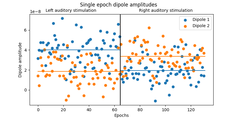
为总结并可视化单试次偶极子幅度,我们将绘制不同实验条件下偶极子平均幅度的详细图。
# Summarize the single epoch timecourses by computing the mean amplitude from
# 60-90ms.
amplitudes_left = []
amplitudes_right = []
for stc in stcs_left:
    amplitudes_left.append(stc.crop(0.06, 0.09).mean().data)
for stc in stcs_right:
    amplitudes_right.append(stc.crop(0.06, 0.09).mean().data)
amplitudes = np.vstack([amplitudes_left, amplitudes_right])

# Visualize the epoch-by-epoch dipole ampltudes in a detailed figure.
n = len(amplitudes)
n_left = len(amplitudes_left)
mean_left = np.mean(amplitudes_left, axis=0)
mean_right = np.mean(amplitudes_right, axis=0)

fig, ax = plt.subplots(figsize=(8, 4))
ax.scatter(np.arange(n), amplitudes[:, 0], label="Dipole 1")
ax.scatter(np.arange(n), amplitudes[:, 1], label="Dipole 2")
transition_point = n_left - 0.5
ax.plot([0, transition_point], [mean_left[0], mean_left[0]], color="C0")
ax.plot([0, transition_point], [mean_left[1], mean_left[1]], color="C1")
ax.plot([transition_point, n], [mean_right[0], mean_right[0]], color="C0")
ax.plot([transition_point, n], [mean_right[1], mean_right[1]], color="C1")
ax.axvline(transition_point, color="black")
ax.set_xlabel("Epochs")
ax.set_ylabel("Dipole amplitude")
ax.legend()
fig.suptitle("Single epoch dipole amplitudes")
fig.text(0.30, 0.9, "Left auditory stimulation", ha="center")
fig.text(0.70, 0.9, "Right auditory stimulation", ha="center")
脚本总运行时间:(0 分 6.974 秒)