非官方中文翻译 本页译自 MNE-Python 官方文档： 查看英文原文 ↗。 文档版权归 MNE Developers 所有（BSD-3-Clause）。

从原始数据中读取阻抗

许多 EEG 系统会在文件格式中提供各通道的阻抗测量值。MNE 不会解析这类信息，也不会将其存入 Raw 对象；不过，仍可以从原始数据中提取这些信息，并保存到单独的数据结构中。

ANT Neuro

ANT Neuro 的 .cnt 文件格式以触发器的形式保存阻抗信息。mne.io.read_raw_ant() 会读取这些信息，并将执行阻抗测量的时间段标记为 Annotations，其描述由参数 impedance_annotation 指定；但它不会提取阻抗数值本身。若需提取数值，请使用 antio.parser.read_triggers。

# Authors: The MNE-Python contributors.
# License: BSD-3-Clause
# Copyright the MNE-Python contributors.

import numpy as np
from antio import read_cnt
from antio.parser import read_triggers
from matplotlib import pyplot as plt
from mffpy.xml_files import DataInfo

from mne.datasets import testing
from mne.io import read_raw_ant, read_raw_egi
from mne.viz import plot_topomap

fname = testing.data_path() / "antio" / "CA_208" / "test_CA_208.cnt"
cnt = read_cnt(fname)
_, _, _, impedances, _ = read_triggers(cnt)

raw = read_raw_ant(fname, eog=r"EOG")
impedances = [{ch: imp[k] for k, ch in enumerate(raw.ch_names)} for imp in impedances]
print(impedances[0])  # impedances measurement at the beginning of the recording

Reading ANT file /home/circleci/mne_data/MNE-testing-data/antio/CA_208/test_CA_208.cnt
All 63 EEG channels are referenced to CPz.
{'Fp1': 2.254, 'Fpz': 2.926, 'Fp2': 2.693, 'F7': 13.045, 'F3': 0.902, 'Fz': 2.737, 'F4': 0.149, 'F8': 25.132999, 'FC5': 0.304, 'FC1': 38.924, 'FC2': 2.258, 'FC6': 0.135, 'M1': 4.445, 'T7': 6.233, 'C3': 8.322, 'Cz': 0.064, 'C4': 1.271, 'T8': 4.049, 'M2': 1.846, 'CP5': 2.721, 'CP1': 2.944, 'CP2': 1.218, 'CP6': 0.879, 'P7': 22.726999, 'P3': 9.176, 'Pz': 1.84, 'P4': 27.167, 'P8': 1.157, 'POz': 3.575, 'O1': 2.698, 'O2': 8.073, 'EOG': 15.205, 'AF7': 5.842, 'AF3': 1.303, 'AF4': 2.136, 'AF8': 0.787, 'F5': 0.863, 'F1': 1.696, 'F2': 1.616, 'F6': 0.478, 'FC3': 6.01, 'FCz': 0.72, 'FC4': 4.314, 'C5': 10.945, 'C1': 6.151, 'C2': 0.772, 'C6': 0.879, 'CP3': 12.115, 'CP4': 1.887, 'P5': 14.045, 'P1': 2.733, 'P2': 34.641998, 'P6': 1.765, 'PO5': 5.666, 'PO3': 14.12, 'PO4': 2.599, 'PO6': 11.339, 'FT7': 13.158, 'FT8': 1.046, 'TP7': 5.917, 'TP8': 2.61, 'PO7': 5.691, 'PO8': 1.759, 'Oz': 5.165, 'BIP1': 2147483.75, 'BIP2': 2147483.75, 'BIP3': 2147483.75, 'BIP4': 2147483.75, 'BIP5': 2147483.75, 'BIP6': 2147483.75, 'BIP7': 2147483.75, 'BIP8': 2147483.75, 'BIP9': 2147483.75, 'BIP10': 2147483.75, 'BIP11': 2147483.75, 'BIP12': 2147483.75, 'BIP13': 2147483.75, 'BIP14': 2147483.75, 'BIP15': 2147483.75, 'BIP16': 2147483.75, 'BIP17': 2147483.75, 'BIP18': 2147483.75, 'BIP19': 2147483.75, 'BIP20': 2147483.75, 'BIP21': 2147483.75, 'BIP22': 2147483.75, 'BIP23': 2147483.75, 'BIP24': 2147483.75}

注意，阻抗测量包含所有通道，包括双极通道。我们可以在地形图上可视化阻抗；下文仅针对 EEG 通道，展示记录前与记录后的阻抗地形图。

raw.pick("eeg").set_montage("colin27_1020")
impedances = [{ch: imp[ch] for ch in raw.ch_names} for imp in impedances]

f, ax = plt.subplots(1, 2, layout="constrained", figsize=(10, 5))
f.suptitle("Impedances (kOhm)")
impedance = list(impedances[0].values())
plot_topomap(
    impedance,
    raw.info,
    vlim=(0, 50),
    axes=ax[0],
    show=False,
    names=[f"{elt:.1f}" for elt in impedance],
)
ax[0].set_title("Impedances at the beginning of the recording")
impedance = list(impedances[-1].values())
plot_topomap(
    impedance,
    raw.info,
    vlim=(0, 50),
    axes=ax[1],
    show=False,
    names=[f"{elt:.1f}" for elt in impedance],
)
ax[1].set_title("Impedances at the end of the recording")
plt.show()

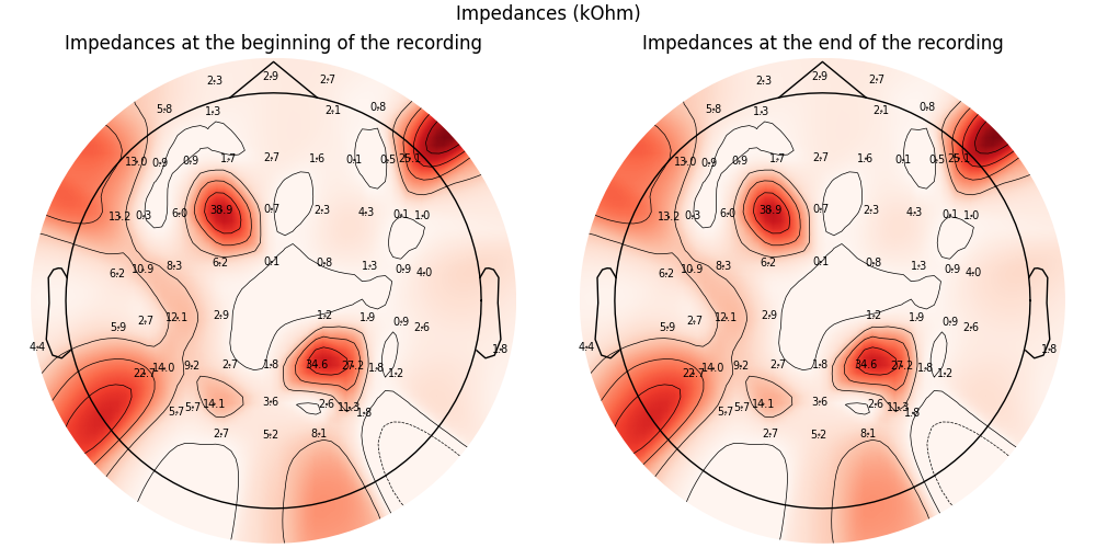
在这个很短的测试文件中，阻抗随时间保持稳定。

EGI

EGI 的 MFF 文件会在 .mff 目录内的 info1.xml 中保存各通道的增益（GCAL）与阻抗（ICAL）校准数据。mne.io.read_raw_egi() 不会在 Raw 对象中提供这些信息，但可以通过 mffpy 直接从 info1.xml 读取。

打开 MFF 文件，仅保留 EEG 通道，然后从 info1.xml 读取校准块。ICAL 条目保存校准时各通道的阻抗值（单位 kΩ）；GCAL 保存各通道的增益校正因子（接近 1.0）。

fname_egi = testing.data_path() / "EGI" / "test_egi.mff"
raw_egi = read_raw_egi(fname_egi, verbose=False)
raw_egi.pick("eeg")

data_info = DataInfo.from_file(fname_egi / "info1.xml")
ical = data_info.calibrations["ICAL"]["channels"]  # 1-indexed dict, values in kΩ

# Channel order in raw matches the 1-indexed calibration keys.
ical_vals = np.array([ical.get(i + 1, np.nan) for i in range(len(raw_egi.ch_names))])
print({ch: round(float(v), 1) for ch, v in zip(raw_egi.ch_names[:5], ical_vals[:5])})

{'E1': 19.8, 'E2': 21.6, 'E3': 18.9, 'E4': 25.3, 'E5': 29.2}

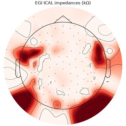
在拓扑图上可视化各通道的 ICAL 阻抗。

fig, ax = plt.subplots(layout="constrained", figsize=(5, 5))
plot_topomap(ical_vals, raw_egi.info, axes=ax, show=False)
ax.set_title("EGI ICAL impedances (kΩ)")
plt.show()