非官方中文翻译 本页译自 MNE-Python 官方文档： 查看英文原文 ↗。 文档版权归 MNE Developers 所有（BSD-3-Clause）。

将 MEG 或 EEG 数据插值到任意电极布局

本示例同时演示 EEG 电极布局插值与 MEG 系统变换。

对 EEG 而言，这有助于在不同数据集之间标准化通道布局（见 [1]）。

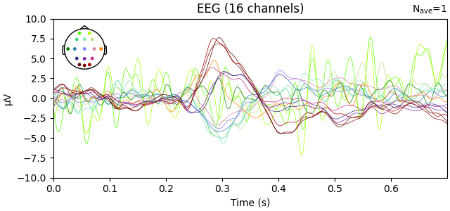
• 对 EEG 数据使用场插值。

• 使用目标电极布局 “biosemi16”。

• 对 MEG 数据使用 MNE 插值，从 Neuromag（平面梯度计与磁强计）变换到 CTF（轴向梯度计）。

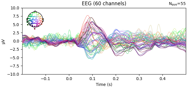
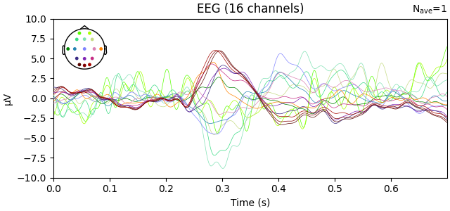
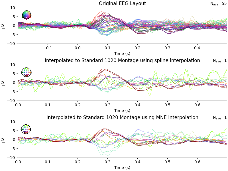
第一个示例把原始 EEG 通道的数据插值到 “biosemi16” 电极布局定义的位置。

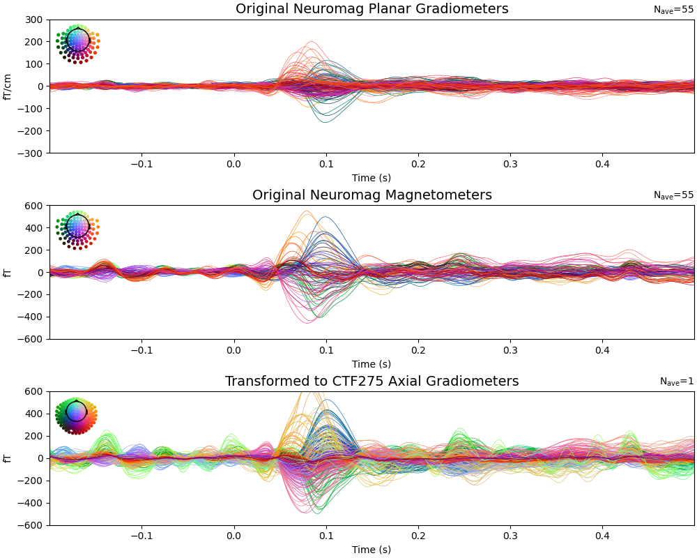
第二个示例把 306 传感器 Neuromag 的 MEG 数据插值到 275 传感器的 CTF 系统。

# Authors: Antoine Collas <contact@antoinecollas.fr>
#          Konstantinos Tsilimparis <konstantinos.tsilimparis@outlook.com>
# License: BSD-3-Clause
# Copyright the MNE-Python contributors.

import matplotlib.pyplot as plt

import mne
from mne.channels import make_standard_montage
from mne.datasets import sample

print(__doc__)
ylim = (-10, 10)

第 1 部分：EEG 系统变换

# Load EEG data
data_path = sample.data_path()
eeg_file_path = data_path / "MEG" / "sample" / "sample_audvis-ave.fif"
evoked = mne.read_evokeds(eeg_file_path, condition="Left Auditory", baseline=(None, 0))

# Select only EEG channels
evoked.pick("eeg")

# Plot the original EEG layout
evoked.plot(exclude=[], picks="eeg", ylim=dict(eeg=ylim))

Reading /home/circleci/mne_data/MNE-sample-data/MEG/sample/sample_audvis-ave.fif ...
    Read a total of 4 projection items:
        PCA-v1 (1 x 102) active
        PCA-v2 (1 x 102) active
        PCA-v3 (1 x 102) active
        Average EEG reference (1 x 60) active
    Found the data of interest:
        t =    -199.80 ...     499.49 ms (Left Auditory)
        0 CTF compensation matrices available
        nave = 55 - aspect type = 100
Projections have already been applied. Setting proj attribute to True.
Applying baseline correction (mode: mean)

定义目标电极布局

standard_montage = make_standard_montage("biosemi16")

使用 interpolate_to 把 EEG 数据投影到标准电极布局

evoked_interpolated_spline = evoked.copy().interpolate_to(
    standard_montage, method="spline"
)

# Plot the interpolated EEG layout
evoked_interpolated_spline.plot(exclude=[], picks="eeg", ylim=dict(eeg=ylim))

Automatic origin fit: head of radius 91.2 mm

使用 interpolate_to 把 EEG 数据投影到标准电极布局

evoked_interpolated_mne = evoked.copy().interpolate_to(standard_montage, method="MNE")

# Plot the interpolated EEG layout
evoked_interpolated_mne.plot(exclude=[], picks="eeg", ylim=dict(eeg=ylim))

Adding average EEG reference projection.
    Automatic origin fit: head of radius 91.2 mm
    Computing dot products for 59 EEG channels...
    Computing cross products for 59 → 16 EEG channels...
    Preparing the mapping matrix...
    Truncating at 58/59 components and regularizing with α=1.0e-01
    The map has an average electrode reference (16 channels)

比较插值前后

fig, axs = plt.subplots(3, 1, figsize=(8, 6), constrained_layout=True)
evoked.plot(exclude=[], picks="eeg", axes=axs[0], show=False, ylim=dict(eeg=ylim))
axs[0].set_title("Original EEG Layout")
evoked_interpolated_spline.plot(
    exclude=[], picks="eeg", axes=axs[1], show=False, ylim=dict(eeg=ylim)
)
axs[1].set_title("Interpolated to Standard 1020 Montage using spline interpolation")
evoked_interpolated_mne.plot(
    exclude=[], picks="eeg", axes=axs[2], show=False, ylim=dict(eeg=ylim)
)
axs[2].set_title("Interpolated to Standard 1020 Montage using MNE interpolation")

第 2 部分：MEG 系统变换

我们演示把 MEG 数据从 Neuromag（平面梯度计与磁强计）变换到 CTF（轴向梯度计）传感器配置。

# Load the full evoked data with MEG channels
evoked_meg = mne.read_evokeds(
    eeg_file_path, condition="Left Auditory", baseline=(None, 0)
)
evoked_meg.pick("meg")

print("Original Neuromag system:")
print(f"  Number of magnetometers: {len(mne.pick_types(evoked_meg.info, meg='mag'))}")
print(f"  Number of gradiometers: {len(mne.pick_types(evoked_meg.info, meg='grad'))}")

Reading /home/circleci/mne_data/MNE-sample-data/MEG/sample/sample_audvis-ave.fif ...
    Read a total of 4 projection items:
        PCA-v1 (1 x 102) active
        PCA-v2 (1 x 102) active
        PCA-v3 (1 x 102) active
        Average EEG reference (1 x 60) active
    Found the data of interest:
        t =    -199.80 ...     499.49 ms (Left Auditory)
        0 CTF compensation matrices available
        nave = 55 - aspect type = 100
Projections have already been applied. Setting proj attribute to True.
Applying baseline correction (mode: mean)
Original Neuromag system:
  Number of magnetometers: 102
  Number of gradiometers: 203

变换到 CTF 传感器配置

# Interpolate Neuromag to CTF
evoked_ctf = evoked_meg.copy().interpolate_to("ctf275", mode="accurate")

print("\nTransformed to CTF system:")
print(f"  Number of MEG channels: {len(mne.pick_types(evoked_ctf.info, meg=True))}")
print(f"  Bad channels in original: {evoked_meg.info['bads']}")

    Automatic origin fit: head of radius 91.2 mm
    Computing dot products for 305 MEG channels...
    Computing cross products for 305 → 274 MEG channels...
    Preparing the mapping matrix...
    Truncating at 85/305 components to omit less than 0.0001 (9.4e-05)

Transformed to CTF system:
  Number of MEG channels: 274
  Bad channels in original: ['MEG 2443']

比较诱发响应：原始 Neuromag 与变换后的 CTF。数据应相似，但投影到不同的传感器阵列。

# Set consistent y-limits for comparison
ylim_meg = dict(grad=[-300, 300], mag=[-600, 600], meg=[-300, 300])

fig, axes = plt.subplots(3, 1, figsize=(10, 8), layout="constrained")

# Plot original Neuromag gradiometers
evoked_meg.copy().pick("grad").plot(
    axes=axes[0], show=False, spatial_colors=True, ylim=ylim_meg, time_unit="s"
)
axes[0].set_title("Original Neuromag Planar Gradiometers", fontsize=14)


# Plot original Neuromag magnetometers
evoked_meg.copy().pick("mag").plot(
    axes=axes[1], show=False, spatial_colors=True, ylim=ylim_meg, time_unit="s"
)
axes[1].set_title("Original Neuromag Magnetometers", fontsize=14)

# Plot transformed CTF gradiometers
evoked_ctf.plot(
    axes=axes[2], show=False, spatial_colors=True, ylim=ylim_meg, time_unit="s"
)
axes[2].set_title("Transformed to CTF275 Axial Gradiometers", fontsize=14)

参考文献

[1]

Apolline Mellot, Antoine Collas, Sylvain Chevallier, Denis Engemann, and Alexandre Gramfort. Physics-informed and unsupervised riemannian domain adaptation for machine learning on heterogeneous eeg datasets. In Proceedings of the 32nd European Signal Processing Conference (EUSIPCO). Lyon, France, 2024.