
非官方中文翻译
本页译自 MNE-Python 官方文档:
查看英文原文 ↗。
文档版权归 MNE Developers 所有(BSD-3-Clause)。
说明
转到末尾下载完整示例代码。
通过 MNE 投影协方差计算源功率估计#
可以把 MNE 逆算子应用于协方差矩阵,得到源功率估计。这比先估计源时间过程再计算其功率在计算上更高效。本代码基于 [1],在预测建模中借助源定位校正个体场扩散时很有用。
参考文献#
# Author: Denis A. Engemann <denis-alexander.engemann@inria.fr>
#         Luke Bloy <luke.bloy@gmail.com>
#
# License: BSD-3-Clause
# Copyright the MNE-Python contributors.
import numpy as np

import mne
from mne.datasets import sample
from mne.minimum_norm import apply_inverse_cov, make_inverse_operator

data_path = sample.data_path()
subjects_dir = data_path / "subjects"
meg_path = data_path / "MEG" / "sample"
raw_fname = meg_path / "sample_audvis_filt-0-40_raw.fif"
raw = mne.io.read_raw_fif(raw_fname)
Opening raw data file /home/circleci/mne_data/MNE-sample-data/MEG/sample/sample_audvis_filt-0-40_raw.fif...
    Read a total of 4 projection items:
        PCA-v1 (1 x 10²)  idle
        PCA-v2 (1 x 10²)  idle
        PCA-v3 (1 x 10²)  idle
        Average EEG reference (1 x 60)  idle
    Range : 6450 ... 48149 =     42.956 ...   320.665 secs
Ready.
计算空室协方差#
首先计算空室协方差,它反映传感器与环境的噪声。
raw_empty_room_fname = data_path / "MEG" / "sample" / "ernoise_raw.fif"
raw_empty_room = mne.io.read_raw_fif(raw_empty_room_fname)
raw_empty_room.crop(0, 30)  # cropped just for speed
raw_empty_room.info["bads"] = ["MEG 2443"]
raw_empty_room.add_proj(raw.info["projs"])
noise_cov = mne.compute_raw_covariance(raw_empty_room, method="shrunk")
del raw_empty_room
Opening raw data file /home/circleci/mne_data/MNE-sample-data/MEG/sample/ernoise_raw.fif...
Isotrak not found
    Read a total of 3 projection items:
        PCA-v1 (1 x 10²)  idle
        PCA-v2 (1 x 10²)  idle
        PCA-v3 (1 x 10²)  idle
    Range : 19800 ... 85867 =     32.966 ...   142.965 secs
Ready.
4 projection items deactivated
Using up to 150 segments
Loading data for 150 events and 120 original time points ...
0 bad epochs dropped
    Created an SSP operator (subspace dimension = 3)
    Setting small MEG eigenvalues to zero (without PCA)
Reducing data rank from 305 -> 302
Estimating covariance using SHRUNK
Done.
Number of samples used : 18000
[done]
对数据分段#
raw.pick(["meg", "stim", "eog"]).load_data().filter(4, 12)
raw.info["bads"] = ["MEG 2443"]
events = mne.find_events(raw, stim_channel="STI 014")
event_id = dict(aud_l=1, aud_r=2, vis_l=3, vis_r=4)
tmin, tmax = -0.2, 0.5
baseline = (None, 0)  # means from the first instant to t = 0
reject = dict(grad=4000e-13, mag=4e-12, eog=150e-6)
epochs = mne.Epochs(
    raw,
    events,
    event_id,
    tmin,
    tmax,
    proj=True,
    picks=("meg", "eog"),
    baseline=None,
    reject=reject,
    preload=True,
    decim=5,
    verbose="error",
)
del raw
Reading 0 ... 41699  =      0.000 ...   277.709 secs...
Filtering raw data in 1 contiguous segment
Setting up band-pass filter from 4 - 12 Hz

FIR filter parameters
---------------------
Designing a one-pass, zero-phase, non-causal bandpass filter:
- Windowed time-domain design (firwin) method
- Hamming window with 0.0194 passband ripple and 53 dB stopband attenuation
- Lower passband edge: 4.00
- Lower transition bandwidth: 2.00 Hz (-6 dB cutoff frequency: 3.00 Hz)
- Upper passband edge: 12.00 Hz
- Upper transition bandwidth: 3.00 Hz (-6 dB cutoff frequency: 13.50 Hz)
- Filter length: 249 samples (1.658 s)

Finding events on: STI 014
319 events found on stim channel STI 014
Event IDs: [ 1  2  3  4  5 32]
计算并绘制协方差#
除上面的空室协方差外,再计算两个协方差:
基线协方差,反映分析中不感兴趣的信号(如传感器噪声、环境噪声、生理伪迹,以及类似静息态的脑活动/“噪声”)。
数据协方差,反映感兴趣的激活(以及噪声源)。
base_cov = mne.compute_covariance(
    epochs, tmin=-0.2, tmax=0, method="shrunk", verbose=True
)
data_cov = mne.compute_covariance(
    epochs, tmin=0.0, tmax=0.2, method="shrunk", verbose=True
)

fig_noise_cov = mne.viz.plot_cov(noise_cov, epochs.info, show_svd=False)
fig_base_cov = mne.viz.plot_cov(base_cov, epochs.info, show_svd=False)
fig_data_cov = mne.viz.plot_cov(data_cov, epochs.info, show_svd=False)
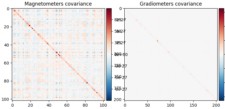
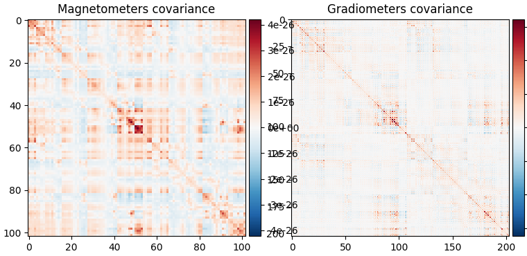
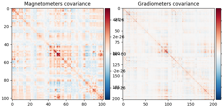
    Created an SSP operator (subspace dimension = 3)
    Setting small MEG eigenvalues to zero (without PCA)
Reducing data rank from 305 -> 302
Estimating covariance using SHRUNK
Done.
Number of samples used : 1680
[done]
    Created an SSP operator (subspace dimension = 3)
    Setting small MEG eigenvalues to zero (without PCA)
Reducing data rank from 305 -> 302
Estimating covariance using SHRUNK
Done.
Number of samples used : 1680
[done]
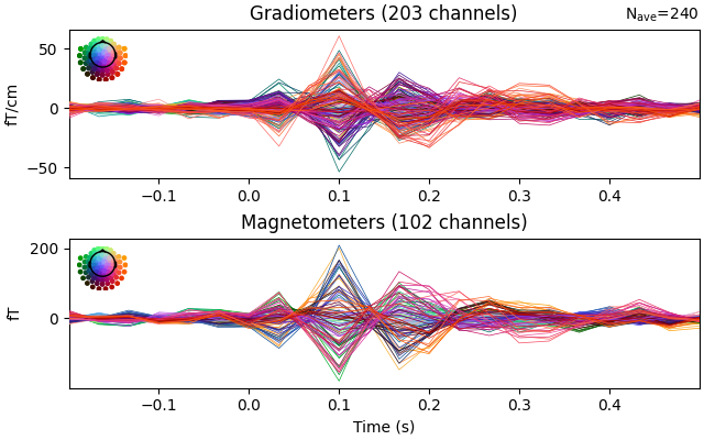
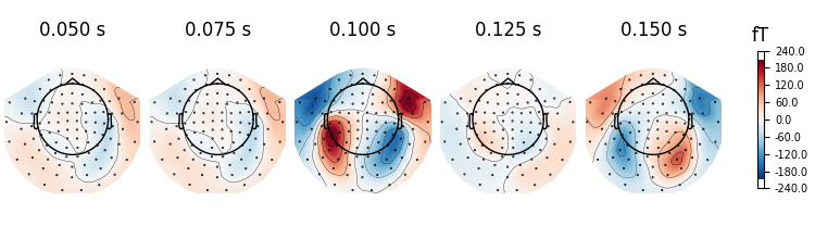
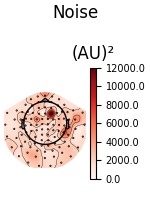
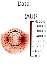
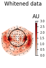
也可以用地形图查看协方差;这里只展示基线协方差与数据协方差,以及用基线协方差白化后的数据协方差:
evoked = epochs.average().pick("meg")
evoked.drop_channels(evoked.info["bads"])
evoked.plot(time_unit="s")
evoked.plot_topomap(times=np.linspace(0.05, 0.15, 5), ch_type="mag")

loop = {
    "Noise": (noise_cov, dict()),
    "Data": (data_cov, dict()),
    "Whitened data": (data_cov, dict(noise_cov=noise_cov)),
}
for title, (_cov, _kw) in loop.items():
    fig = _cov.plot_topomap(evoked.info, "grad", **_kw)
    fig.suptitle(title)
    Created an SSP operator (subspace dimension = 3)
Computing rank from covariance with rank=None
    Using tolerance 1.4e-13 (2.2e-16 eps * 305 dim * 2.1  max singular value)
    Estimated rank (mag + grad): 302
    MEG: rank 302 computed from 305 data channels with 3 projectors
    Setting small MEG eigenvalues to zero (without PCA)
    Created the whitener using a noise covariance matrix with rank 302 (3 small eigenvalues omitted)
对协方差应用逆算子#
最后,可用空室噪声协方差构建逆算子:
# Read the forward solution and compute the inverse operator
fname_fwd = meg_path / "sample_audvis-meg-oct-6-fwd.fif"
fwd = mne.read_forward_solution(fname_fwd)
# make an MEG inverse operator
info = evoked.info
inverse_operator = make_inverse_operator(info, fwd, noise_cov, loose=0.2, depth=0.8)
Reading forward solution from /home/circleci/mne_data/MNE-sample-data/MEG/sample/sample_audvis-meg-oct-6-fwd.fif...
    Reading a source space...
    Computing patch statistics...
    Patch information added...
    Distance information added...
    [done]
    Reading a source space...
    Computing patch statistics...
    Patch information added...
    Distance information added...
    [done]
    2 source spaces read
    Desired named matrix (kind = 3523 (FIFF_MNE_FORWARD_SOLUTION_GRAD)) not available
    Read MEG forward solution (7498 sources, 306 channels, free orientations)
    Source spaces transformed to the forward solution coordinate frame
Converting forward solution to surface orientation
    Average patch normals will be employed in the rotation to the local surface coordinates....
    Converting to surface-based source orientations...
    [done]
Computing inverse operator with 305 channels.
    305 out of 306 channels remain after picking
Selected 305 channels
Creating the depth weighting matrix...
    203 planar channels
    limit = 7265/7498 = 10.037795
    scale = 2.52065e-08 exp = 0.8
Applying loose dipole orientations to surface source spaces: 0.2
Whitening the forward solution.
    Created an SSP operator (subspace dimension = 3)
Computing rank from covariance with rank=None
    Using tolerance 1.4e-13 (2.2e-16 eps * 305 dim * 2.1  max singular value)
    Estimated rank (mag + grad): 302
    MEG: rank 302 computed from 305 data channels with 3 projectors
    Setting small MEG eigenvalues to zero (without PCA)
Creating the source covariance matrix
Adjusting source covariance matrix.
Computing SVD of whitened and weighted lead field matrix.
    largest singular value = 6.411
    scaling factor to adjust the trace = 5.63162e+19 (nchan = 305 nzero = 3)
把数据与基线协方差投影到源空间:
stc_data = apply_inverse_cov(
    data_cov,
    evoked.info,
    inverse_operator,
    nave=len(epochs),
    method="dSPM",
    verbose=True,
)
stc_base = apply_inverse_cov(
    base_cov,
    evoked.info,
    inverse_operator,
    nave=len(epochs),
    method="dSPM",
    verbose=True,
)
Preparing the inverse operator for use...
    Scaled noise and source covariance from nave = 1 to nave = 240
    Created the regularized inverter
    Created an SSP operator (subspace dimension = 3)
    Created the whitener using a noise covariance matrix with rank 302 (3 small eigenvalues omitted)
    Computing noise-normalization factors (dSPM)...
[done]
Applying inverse operator to "cov"...
    Picked 305 channels from the data
    Computing inverse...
    Eigenleads need to be weighted ...
    Computing residual...
    Explained  37.1% variance
    dSPM...
    Combining the current components...
[done]
并可视化相对于基线的功率:
stc_data /= stc_base
brain = stc_data.plot(
    subject="sample",
    subjects_dir=subjects_dir,
    clim=dict(kind="percent", lims=(50, 90, 98)),
    smoothing_steps=7,
)
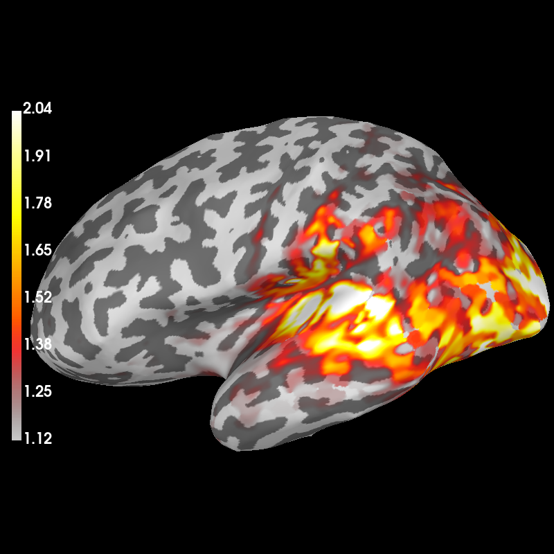
Using control points [1.11813641 1.45873675 2.03828176]
脚本总运行时间:(0 分 12.327 秒)