
非官方中文翻译
本页译自 MNE-Python 官方文档:
查看英文原文 ↗。
文档版权归 MNE Developers 所有(BSD-3-Clause)。
说明
转到末尾下载完整示例代码。
使用环形图可视化标签间的源泄漏#
本示例基于 MNE 逆解与 FreeSurfer 皮层分区,计算源空间中 68 个区域之间的两两泄漏。标签间泄漏以各标签点扩散函数(PSF)之间的相关性估计,并用环形图可视化,环形图按各区域在轴状面上的位置排序。
# Authors: Olaf Hauk <olaf.hauk@mrc-cbu.cam.ac.uk>
#          Martin Luessi <mluessi@nmr.mgh.harvard.edu>
#          Alexandre Gramfort <alexandre.gramfort@inria.fr>
#          Nicolas P. Rougier (graph code borrowed from his matplotlib gallery)
#
# License: BSD-3-Clause
# Copyright the MNE-Python contributors.
import matplotlib.pyplot as plt
import numpy as np
from mne_connectivity.viz import plot_connectivity_circle

import mne
from mne.datasets import sample
from mne.minimum_norm import (
    get_point_spread,
    make_inverse_resolution_matrix,
    read_inverse_operator,
)
from mne.viz import circular_layout

print(__doc__)
加载正向解与逆算子#
需要匹配的正向解与逆算子,才能计算不同方法的分辨率矩阵。
data_path = sample.data_path()
subjects_dir = data_path / "subjects"
meg_path = data_path / "MEG" / "sample"
fname_fwd = meg_path / "sample_audvis-meg-eeg-oct-6-fwd.fif"
fname_inv = meg_path / "sample_audvis-meg-oct-6-meg-fixed-inv.fif"
forward = mne.read_forward_solution(fname_fwd)
# Convert forward solution to fixed source orientations
mne.convert_forward_solution(forward, surf_ori=True, force_fixed=True, copy=False)
inverse_operator = read_inverse_operator(fname_inv)

# Compute resolution matrices for MNE
rm_mne = make_inverse_resolution_matrix(
    forward, inverse_operator, method="MNE", lambda2=1.0 / 3.0**2
)
src = inverse_operator["src"]
del forward, inverse_operator  # save memory
Reading forward solution from /home/circleci/mne_data/MNE-sample-data/MEG/sample/sample_audvis-meg-eeg-oct-6-fwd.fif...
    Reading a source space...
    Computing patch statistics...
    Patch information added...
    Distance information added...
    [done]
    Reading a source space...
    Computing patch statistics...
    Patch information added...
    Distance information added...
    [done]
    2 source spaces read
    Desired named matrix (kind = 3523 (FIFF_MNE_FORWARD_SOLUTION_GRAD)) not available
    Read MEG forward solution (7498 sources, 306 channels, free orientations)
    Desired named matrix (kind = 3523 (FIFF_MNE_FORWARD_SOLUTION_GRAD)) not available
    Read EEG forward solution (7498 sources, 60 channels, free orientations)
    Forward solutions combined: MEG, EEG
    Source spaces transformed to the forward solution coordinate frame
    Average patch normals will be employed in the rotation to the local surface coordinates....
    Converting to surface-based source orientations...
    [done]
Reading inverse operator decomposition from /home/circleci/mne_data/MNE-sample-data/MEG/sample/sample_audvis-meg-oct-6-meg-fixed-inv.fif...
    Reading inverse operator info...
    [done]
    Reading inverse operator decomposition...
    [done]
    305 x 305 full covariance (kind = 1) found.
    Read a total of 4 projection items:
        PCA-v1 (1 x 10²) active
        PCA-v2 (1 x 10²) active
        PCA-v3 (1 x 10²) active
        Average EEG reference (1 x 60) active
    Noise covariance matrix read.
    7498 x 7498 diagonal covariance (kind = 2) found.
    Source covariance matrix read.
    Did not find the desired covariance matrix (kind = 6)
    7498 x 7498 diagonal covariance (kind = 5) found.
    Depth priors read.
    Did not find the desired covariance matrix (kind = 3)
    Reading a source space...
    Computing patch statistics...
    Patch information added...
    Distance information added...
    [done]
    Reading a source space...
    Computing patch statistics...
    Patch information added...
    Distance information added...
    [done]
    2 source spaces read
    Read a total of 4 projection items:
        PCA-v1 (1 x 10²) active
        PCA-v2 (1 x 10²) active
        PCA-v3 (1 x 10²) active
        Average EEG reference (1 x 60) active
    Source spaces transformed to the inverse solution coordinate frame
    305 out of 366 channels remain after picking
Preparing the inverse operator for use...
    Scaled noise and source covariance from nave = 1 to nave = 1
    Created the regularized inverter
    Created an SSP operator (subspace dimension = 3)
    Created the whitener using a noise covariance matrix with rank 302 (3 small eigenvalues omitted)
Applying inverse operator to ""...
    Picked 305 channels from the data
    Computing inverse...
    Eigenleads need to be weighted ...
    Computing residual...
    Explained  44.6% variance
[done]
Dimension of Inverse Matrix: (7498, 305)
Dimensions of resolution matrix: 7498 by 7498.
读取并整理皮层分区的标签#
获取 FreeSurfer ‘aparc’ 皮层分区的标签,每个半球 34 个
labels = mne.read_labels_from_annot("sample", parc="aparc", subjects_dir=subjects_dir)
n_labels = len(labels)
label_colors = [label.color for label in labels]
# First, we reorder the labels based on their location in the left hemi
label_names = [label.name for label in labels]
lh_labels = [name for name in label_names if name.endswith("lh")]

# Get the y-location of the label
label_ypos = list()
for name in lh_labels:
    idx = label_names.index(name)
    ypos = np.mean(labels[idx].pos[:, 1])
    label_ypos.append(ypos)

# Reorder the labels based on their location
lh_labels = [label for (yp, label) in sorted(zip(label_ypos, lh_labels))]

# For the right hemi
rh_labels = [label[:-2] + "rh" for label in lh_labels]
Reading labels from parcellation...
   read 34 labels from /home/circleci/mne_data/MNE-sample-data/subjects/sample/label/lh.aparc.annot
   read 34 labels from /home/circleci/mne_data/MNE-sample-data/subjects/sample/label/rh.aparc.annot
为所有标签计算点扩散函数汇总(PCA)#
用每个标签 PSF 的前五个主成分做汇总,并用第一主成分评估下面的标签间泄漏。
# Compute first PCA component across PSFs within labels.
# Note the differences in explained variance, probably due to different
# spatial extents of labels.
n_comp = 5
stcs_psf_mne, pca_vars_mne = get_point_spread(
    rm_mne, src, labels, mode="svd", n_comp=n_comp, norm=None, return_pca_vars=True
)
n_verts = rm_mne.shape[0]
del rm_mne
可以显示各标签主成分的解释方差。注意它们因标签空间范围不同而有所差异。
with np.printoptions(precision=1):
    for [name, var] in zip(label_names, pca_vars_mne):
        print(f"{name}: {var.sum():.1f}% {var}")
bankssts-lh: 94.1% [41.1 33.4 10.8  5.4  3.5]
bankssts-rh: 94.7% [56.7 15.8 14.3  4.5  3.4]
caudalanteriorcingulate-lh: 97.9% [72.7 14.8  5.2  3.5  1.7]
caudalanteriorcingulate-rh: 96.8% [63.4 18.7  9.3  3.   2.4]
caudalmiddlefrontal-lh: 91.8% [35.7 25.5 14.9  8.2  7.4]
caudalmiddlefrontal-rh: 90.3% [30.2 27.5 15.9  9.3  7.3]
cuneus-lh: 95.1% [40.6 28.9 17.1  5.7  2.8]
cuneus-rh: 94.4% [39.1 32.5 15.8  3.8  3.3]
entorhinal-lh: 98.6% [52.6 27.5 10.2  6.3  2.1]
entorhinal-rh: 99.6% [48.8 37.1 12.2  0.9  0.6]
frontalpole-lh: 99.9% [70.  22.8  3.5  3.1  0.5]
frontalpole-rh: 99.8% [69.1 24.8  3.3  2.1  0.6]
fusiform-lh: 89.4% [37.9 23.  16.4  6.7  5.4]
fusiform-rh: 88.8% [32.1 28.5 15.6  6.9  5.7]
inferiorparietal-lh: 79.8% [24.1 19.1 16.9 11.2  8.5]
inferiorparietal-rh: 79.5% [24.5 17.6 16.  11.8  9.7]
inferiortemporal-lh: 85.2% [27.  22.9 15.8 11.9  7.8]
inferiortemporal-rh: 87.4% [31.8 23.2 16.3  8.4  7.7]
insula-lh: 89.9% [34.7 29.1 12.4  9.6  4. ]
insula-rh: 91.8% [39.9 26.  11.9 10.5  3.5]
isthmuscingulate-lh: 98.1% [50.4 35.3  6.1  3.9  2.4]
isthmuscingulate-rh: 97.8% [48.6 36.   7.6  3.6  2.1]
lateraloccipital-lh: 83.5% [26.4 21.  15.6 12.4  8.1]
lateraloccipital-rh: 79.4% [23.6 22.  15.1 11.1  7.6]
lateralorbitofrontal-lh: 94.2% [46.8 24.3 10.3  7.4  5.4]
lateralorbitofrontal-rh: 94.8% [44.6 26.1 13.9  5.9  4.3]
lingual-lh: 95.7% [46.8 29.5  9.5  7.8  2. ]
lingual-rh: 95.3% [53.5 27.7  7.7  4.   2.4]
medialorbitofrontal-lh: 91.8% [46.1 23.1 13.5  4.6  4.4]
medialorbitofrontal-rh: 96.5% [58.5 18.3 13.6  3.9  2.1]
middletemporal-lh: 79.5% [30.8 16.4 14.7 10.3  7.4]
middletemporal-rh: 78.9% [30.9 15.9 14.9  9.5  7.8]
paracentral-lh: 95.1% [36.6 35.2 12.8  7.3  3.2]
paracentral-rh: 93.3% [37.2 29.7 11.6 11.   3.7]
parahippocampal-lh: 96.9% [49.5 30.  11.9  3.2  2.4]
parahippocampal-rh: 98.8% [69.4 16.2  9.8  2.6  0.9]
parsopercularis-lh: 93.9% [38.8 34.  11.1  5.5  4.5]
parsopercularis-rh: 95.6% [37.6 33.8 14.9  5.   4.3]
parsorbitalis-lh: 97.5% [51.8 27.2 12.2  4.3  1.9]
parsorbitalis-rh: 98.1% [56.3 25.3  9.5  4.7  2.3]
parstriangularis-lh: 96.6% [54.1 25.7 11.3  3.1  2.5]
parstriangularis-rh: 96.1% [39.6 34.3 13.   6.5  2.6]
pericalcarine-lh: 95.7% [42.5 34.4  9.1  6.4  3.3]
pericalcarine-rh: 95.4% [44.6 34.8  9.1  4.   3. ]
postcentral-lh: 67.3% [16.7 14.5 13.4 12.8 10. ]
postcentral-rh: 65.8% [17.2 14.2 13.5 11.4  9.5]
posteriorcingulate-lh: 98.0% [54.7 31.   7.4  3.3  1.6]
posteriorcingulate-rh: 97.9% [58.4 25.   9.1  3.5  1.8]
precentral-lh: 64.3% [17.8 14.2 12.5 10.7  9.2]
precentral-rh: 63.0% [18.  14.1 11.2 10.8  8.9]
precuneus-lh: 90.5% [43.9 22.9 11.7  6.3  5.7]
precuneus-rh: 84.2% [27.2 25.9 17.1  8.2  5.9]
rostralanteriorcingulate-lh: 97.2% [53.6 22.9 12.4  5.4  2.9]
rostralanteriorcingulate-rh: 98.0% [53.6 25.2 12.2  4.9  2.1]
rostralmiddlefrontal-lh: 69.0% [17.7 15.2 14.7 11.5  9.8]
rostralmiddlefrontal-rh: 70.2% [19.7 15.5 14.3 10.7  9.9]
superiorfrontal-lh: 62.5% [16.1 15.  13.3  9.3  8.8]
superiorfrontal-rh: 61.9% [16.9 14.4 12.8  9.2  8.5]
superiorparietal-lh: 68.3% [18.4 15.2 14.6 11.2  8.9]
superiorparietal-rh: 67.2% [20.3 15.4 12.7 10.3  8.7]
superiortemporal-lh: 86.2% [29.1 19.3 15.9 14.6  7.4]
superiortemporal-rh: 86.3% [29.1 22.  16.2 12.6  6.4]
supramarginal-lh: 84.1% [28.2 21.9 15.9  9.5  8.7]
supramarginal-rh: 85.0% [28.2 22.4 16.7  9.3  8.4]
temporalpole-lh: 98.7% [53.8 33.6  6.8  3.8  0.8]
temporalpole-rh: 99.5% [76.8 16.8  4.5  0.9  0.6]
transversetemporal-lh: 99.0% [76.4 14.9  5.   1.8  1. ]
transversetemporal-rh: 98.4% [50.6 36.5  7.1  2.6  1.5]
输出显示前五个主成分解释的方差总和,以及各成分各自的解释方差。
基于标签间 PSF 相关评估泄漏#
注意相关性忽略 PSF 的总体幅度,即不能说明哪个区域可能是更大的“泄漏者”。
# get PSFs from Source Estimate objects into matrix
psfs_mat = np.zeros([n_labels, n_verts])
# Leakage matrix for MNE, get first principal component per label
for [i, s] in enumerate(stcs_psf_mne):
    psfs_mat[i, :] = s.data[:, 0]
# Compute label-to-label leakage as Pearson correlation of PSFs
# Sign of correlation is arbitrary, so take absolute values
leakage_mne = np.abs(np.corrcoef(psfs_mat))

# Save the plot order and create a circular layout
node_order = lh_labels[::-1] + rh_labels  # mirror label order across hemis
node_angles = circular_layout(
    label_names, node_order, start_pos=90, group_boundaries=[0, len(label_names) / 2]
)
# Plot the graph using node colors from the FreeSurfer parcellation. We only
# show the 200 strongest connections.
fig, ax = plt.subplots(
    figsize=(8, 8), facecolor="black", subplot_kw=dict(projection="polar")
)
plot_connectivity_circle(
    leakage_mne,
    label_names,
    n_lines=200,
    node_angles=node_angles,
    node_colors=label_colors,
    title="MNE Leakage",
    ax=ax,
)
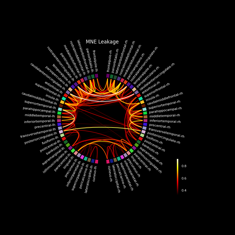
泄漏主要发生在相邻区域之间,但跨半球的深部区域之间也会出现。
保存图像(可选)#
Matplotlib 对交互显示与保存图像分别控制图形背景色。因此保存时必须指定 facecolor,否则标签、标题等将不可见:
绘制单个标签的 PSF#
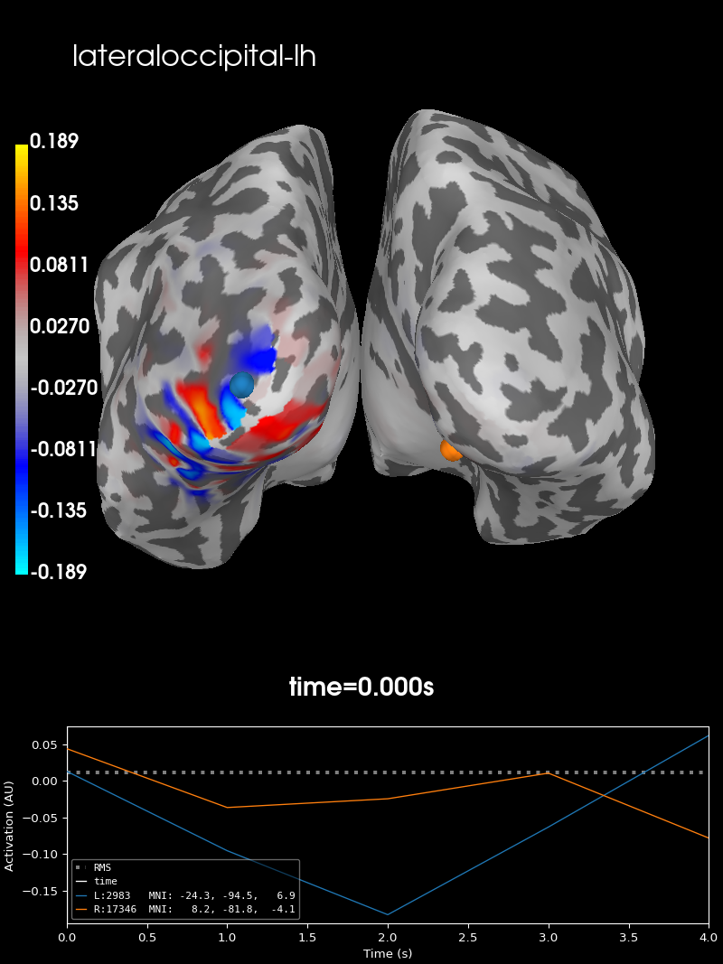
我们确认左右外侧枕叶之间确实没有泄漏,正如相关图所示。可以绘制两个标签的汇总 PSF,检查其泄漏的空间范围。
# left and right lateral occipital
idx = [22, 23]
stc_lh = stcs_psf_mne[idx[0]]
stc_rh = stcs_psf_mne[idx[1]]

# Maximum for scaling across plots
max_val = np.max([stc_lh.data, stc_rh.data])
左半球外侧枕叶标签的点扩散函数
brain_lh = stc_lh.plot(
    subjects_dir=subjects_dir,
    subject="sample",
    hemi="both",
    views="caudal",
    clim=dict(kind="value", pos_lims=(0, max_val / 2.0, max_val)),
)
brain_lh.add_text(0.1, 0.9, label_names[idx[0]], "title", font_size=16)
以及右半球。
brain_rh = stc_rh.plot(
    subjects_dir=subjects_dir,
    subject="sample",
    hemi="both",
    views="caudal",
    clim=dict(kind="value", pos_lims=(0, max_val / 2.0, max_val)),
)
brain_rh.add_text(0.1, 0.9, label_names[idx[1]], "title", font_size=16)
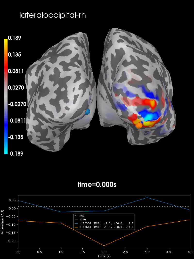
两个汇总 PSF 都局限在各自半球内,说明这两个区域之间确实泄漏很低。
脚本总运行时间:(0 分 8.457 秒)