非官方中文翻译 本页译自 MNE-Python 官方文档： 查看英文原文 ↗。 文档版权归 MNE Developers 所有（BSD-3-Clause）。

偶极子方向在分布式源定位中的作用

在进行分布式源定位（即使用 MNE/dSPM/sLORETA/eLORETA）时，源空间被定义为一个覆盖大部分皮层区域的偶极子网格。这些偶极子既有位置，也有方向。本教程将介绍限制偶极子方向的各种可用选项，以及这些选项对最终源估计结果的影响。

警告

一个常见的“坑”是：默认情况下，源估计会丢弃偶极子方向信息，只保留活动的幅值。这意味着默认得到的源水平数值始终为正，这会带来一些可能并不那么直观的影响：

• 对源估计后的各个 epoch 求平均并不会得到源估计的诱发响应。由于数值始终为正，噪声不会相互“抵消”。这意味着默认设置可能不适合在源空间中对 epoch 进行线性回归或计算相关性等操作。

• 振荡信号会被扭曲，例如正弦波会变成一连串的凸起。因此，在使用默认设置时，在源空间中进行频率分析是没有意义的。

相关信息请参阅 Orientation constraints。

# Authors: The MNE-Python contributors.
# License: BSD-3-Clause
# Copyright the MNE-Python contributors.

加载数据

加载在示例数据集上进行源定位所需的全部内容。

import numpy as np

import mne
from mne.datasets import sample
from mne.minimum_norm import apply_inverse, make_inverse_operator

data_path = sample.data_path()
meg_path = data_path / "MEG" / "sample"
evokeds = mne.read_evokeds(meg_path / "sample_audvis-ave.fif")
left_auditory = evokeds[0].apply_baseline()
fwd = mne.read_forward_solution(meg_path / "sample_audvis-meg-eeg-oct-6-fwd.fif")
mne.convert_forward_solution(fwd, surf_ori=True, copy=False)
noise_cov = mne.read_cov(meg_path / "sample_audvis-cov.fif")
subject = "sample"
subjects_dir = data_path / "subjects"
trans_fname = meg_path / "sample_audvis_raw-trans.fif"

Reading /home/circleci/mne_data/MNE-sample-data/MEG/sample/sample_audvis-ave.fif ...
    Read a total of 4 projection items:
        PCA-v1 (1 x 102) active
        PCA-v2 (1 x 102) active
        PCA-v3 (1 x 102) active
        Average EEG reference (1 x 60) active
    Found the data of interest:
        t =    -199.80 ...     499.49 ms (Left Auditory)
        0 CTF compensation matrices available
        nave = 55 - aspect type = 100
Projections have already been applied. Setting proj attribute to True.
No baseline correction applied
    Read a total of 4 projection items:
        PCA-v1 (1 x 102) active
        PCA-v2 (1 x 102) active
        PCA-v3 (1 x 102) active
        Average EEG reference (1 x 60) active
    Found the data of interest:
        t =    -199.80 ...     499.49 ms (Right Auditory)
        0 CTF compensation matrices available
        nave = 61 - aspect type = 100
Projections have already been applied. Setting proj attribute to True.
No baseline correction applied
    Read a total of 4 projection items:
        PCA-v1 (1 x 102) active
        PCA-v2 (1 x 102) active
        PCA-v3 (1 x 102) active
        Average EEG reference (1 x 60) active
    Found the data of interest:
        t =    -199.80 ...     499.49 ms (Left visual)
        0 CTF compensation matrices available
        nave = 67 - aspect type = 100
Projections have already been applied. Setting proj attribute to True.
No baseline correction applied
    Read a total of 4 projection items:
        PCA-v1 (1 x 102) active
        PCA-v2 (1 x 102) active
        PCA-v3 (1 x 102) active
        Average EEG reference (1 x 60) active
    Found the data of interest:
        t =    -199.80 ...     499.49 ms (Right visual)
        0 CTF compensation matrices available
        nave = 58 - aspect type = 100
Projections have already been applied. Setting proj attribute to True.
No baseline correction applied
Applying baseline correction (mode: mean)
Reading forward solution from /home/circleci/mne_data/MNE-sample-data/MEG/sample/sample_audvis-meg-eeg-oct-6-fwd.fif...
    Reading a source space...
    Computing patch statistics...
    Patch information added...
    Distance information added...
    [done]
    Reading a source space...
    Computing patch statistics...
    Patch information added...
    Distance information added...
    [done]
    2 source spaces read
    Desired named matrix (kind = 3523 (FIFF_MNE_FORWARD_SOLUTION_GRAD)) not available
    Read MEG forward solution (7498 sources, 306 channels, free orientations)
    Desired named matrix (kind = 3523 (FIFF_MNE_FORWARD_SOLUTION_GRAD)) not available
    Read EEG forward solution (7498 sources, 60 channels, free orientations)
    Forward solutions combined: MEG, EEG
    Source spaces transformed to the forward solution coordinate frame
    Average patch normals will be employed in the rotation to the local surface coordinates....
    Converting to surface-based source orientations...
    [done]
    366 x 366 full covariance (kind = 1) found.
    Read a total of 4 projection items:
        PCA-v1 (1 x 102) active
        PCA-v2 (1 x 102) active
        PCA-v3 (1 x 102) active
        Average EEG reference (1 x 60) active

源空间

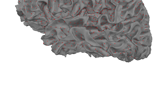
首先来看由 mne.setup_source_space() 函数构建的源空间。偶极子按固定的间隔放置在皮层上，间隔由 spacing 参数决定。源空间并不定义这些偶极子的方向。

lh = fwd["src"][0]  # Visualize the left hemisphere
verts = lh["rr"]  # The vertices of the source space
tris = lh["tris"]  # Groups of three vertices that form triangles
dip_pos = lh["rr"][lh["vertno"]]  # The position of the dipoles
dip_ori = lh["nn"][lh["vertno"]]
dip_len = len(dip_pos)
dip_times = [0]
white = (1.0, 1.0, 1.0)  # RGB values for a white color

actual_amp = np.ones(dip_len)  # fake amp, needed to create Dipole instance
actual_gof = np.ones(dip_len)  # fake GOF, needed to create Dipole instance
dipoles = mne.Dipole(dip_times, dip_pos, actual_amp, dip_ori, actual_gof)
trans = mne.read_trans(trans_fname)

fig = mne.viz.create_3d_figure(size=(600, 400), bgcolor=white)
coord_frame = "mri"

# Plot the cortex
mne.viz.plot_alignment(
    subject=subject,
    subjects_dir=subjects_dir,
    trans=trans,
    surfaces="white",
    coord_frame=coord_frame,
    fig=fig,
)

# Mark the position of the dipoles with small red dots
mne.viz.plot_dipole_locations(
    dipoles=dipoles,
    trans=trans,
    mode="sphere",
    subject=subject,
    subjects_dir=subjects_dir,
    coord_frame=coord_frame,
    scale=7e-4,
    fig=fig,
)

mne.viz.set_3d_view(figure=fig, azimuth=180, distance=0.1, focalpoint="auto")

固定偶极子方向

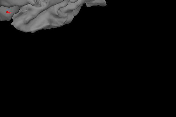
源空间定义偶极子的位置，而逆算子定义它们可能的方向。其中一种选项是为偶极子指定固定方向。由于产生 MEG 和 EEG 信号的神经电流大多垂直于皮层流动 [ 1 ]，因此相应地限制偶极子方向可为源估计提供一个有用的约束。

在调用 mne.minimum_norm.make_inverse_operator() 时指定 fixed=True，偶极子方向就会被固定为垂直于皮层表面并朝外。下面我们将其可视化：

fig = mne.viz.create_3d_figure(size=(600, 400))

# Plot the cortex
mne.viz.plot_alignment(
    subject=subject,
    subjects_dir=subjects_dir,
    trans=trans,
    surfaces="white",
    coord_frame="head",
    fig=fig,
)

# Show the dipoles as arrows pointing along the surface normal
mne.viz.plot_dipole_locations(
    dipoles=dipoles,
    trans=trans,
    mode="arrow",
    subject=subject,
    subjects_dir=subjects_dir,
    coord_frame="head",
    scale=7e-4,
    fig=fig,
)

mne.viz.set_3d_view(figure=fig, azimuth=180, distance=0.1, focalpoint="auto")

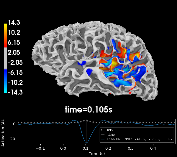
以这种方式限制偶极子方向后，示例数据得到的源估计如下：

# Compute the source estimate for the left auditory condition in the sample
# dataset.
inv = make_inverse_operator(left_auditory.info, fwd, noise_cov, fixed=True)
stc = apply_inverse(left_auditory, inv, pick_ori=None)

# Visualize it at the moment of peak activity.
_, time_max = stc.get_peak(hemi="lh")
brain_fixed = stc.plot(
    surface="white",
    subjects_dir=subjects_dir,
    initial_time=time_max,
    time_unit="s",
    size=(600, 400),
)
mne.viz.set_3d_view(figure=brain_fixed, focalpoint=(0.0, 0.0, 50))

Computing inverse operator with 364 channels.
    364 out of 366 channels remain after picking
Selected 364 channels
Creating the depth weighting matrix...
    203 planar channels
    limit = 7262/7498 = 10.020865
    scale = 2.58122e-08 exp = 0.8
    Picked elements from a free-orientation depth-weighting prior into the fixed-orientation one
    Average patch normals will be employed in the rotation to the local surface coordinates....
    Converting to surface-based source orientations...
    [done]
Whitening the forward solution.
    Created an SSP operator (subspace dimension = 4)
Computing rank from covariance with rank=None
    Using tolerance 3.3e-13 (2.2e-16 eps * 305 dim * 4.8  max singular value)
    Estimated rank (mag + grad): 302
    MEG: rank 302 computed from 305 data channels with 3 projectors
    Using tolerance 4.7e-14 (2.2e-16 eps * 59 dim * 3.6  max singular value)
    Estimated rank (eeg): 58
    EEG: rank 58 computed from 59 data channels with 1 projector
    Setting small MEG eigenvalues to zero (without PCA)
    Setting small EEG eigenvalues to zero (without PCA)
Creating the source covariance matrix
Adjusting source covariance matrix.
Computing SVD of whitened and weighted lead field matrix.
    largest singular value = 5.70263
    scaling factor to adjust the trace = 1.18949e+19 (nchan = 364 nzero = 4)
Preparing the inverse operator for use...
    Scaled noise and source covariance from nave = 1 to nave = 55
    Created the regularized inverter
    Created an SSP operator (subspace dimension = 4)
    Created the whitener using a noise covariance matrix with rank 360 (4 small eigenvalues omitted)
    Computing noise-normalization factors (dSPM)...
[done]
Applying inverse operator to "Left Auditory"...
    Picked 364 channels from the data
    Computing inverse...
    Eigenleads need to be weighted ...
    Computing residual...
    Explained  64.5% variance
    dSPM...
[done]
Using control points [ 4.06165525  4.70033915 14.34794621]

此时估计电流的方向被限制为两个方向：向内和向外。图中蓝色区域表示电流向内流动，红色区域表示电流向外流动。由于皮层存在曲率，成组的偶极子往往指向相同的方向，即传感器所拾取的电磁场方向。

松散偶极子方向

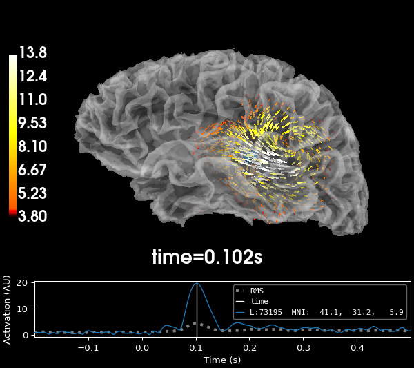
强制源偶极子严格垂直于皮层，会使源估计对偶极子在皮层上的间距变得敏感，因为每个约 10 平方毫米的斑块内皮层曲率都会发生变化。此外，当源偶极子方向受到严格约束时，MEG/EEG 与 MRI 坐标系之间的错位会更加关键 [ 2 ]。为了解除对偶极子方向的限制，逆算子可以在源空间定义的每个位置放置三个而非一个偶极子。这三个偶极子相互正交，构成一个笛卡尔坐标系。下面我们将其可视化：

fig = mne.viz.create_3d_figure(size=(600, 400))

# Plot the cortex
mne.viz.plot_alignment(
    subject=subject,
    subjects_dir=subjects_dir,
    trans=trans,
    surfaces="white",
    coord_frame="head",
    fig=fig,
)

# Show the three dipoles defined at each location in the source space
mne.viz.plot_alignment(
    subject=subject,
    subjects_dir=subjects_dir,
    trans=trans,
    fwd=fwd,
    surfaces="white",
    coord_frame="head",
    fig=fig,
)

mne.viz.set_3d_view(figure=fig, azimuth=180, distance=0.1, focalpoint="auto")

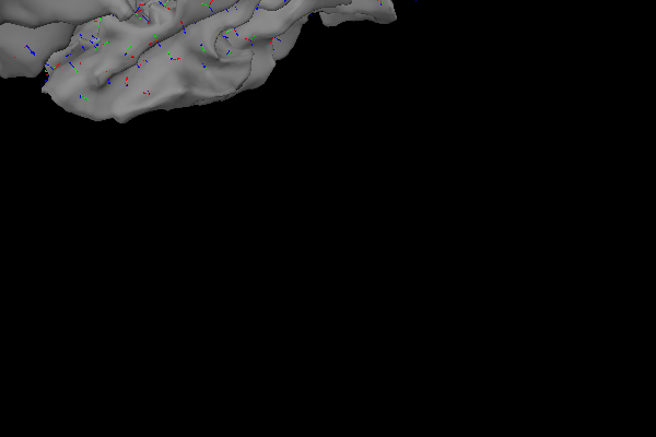
计算源估计时，三个偶极子上的活动会被合并为单个向量的 XYZ 分量，从而得到示例数据的如下源估计：

# Make an inverse operator with loose dipole orientations
inv = make_inverse_operator(left_auditory.info, fwd, noise_cov, fixed=False, loose=1.0)

# Compute the source estimate, indicate that we want a vector solution
stc = apply_inverse(left_auditory, inv, pick_ori="vector")

# Visualize it at the moment of peak activity.
_, time_max = stc.magnitude().get_peak(hemi="lh")
brain_mag = stc.plot(
    subjects_dir=subjects_dir,
    initial_time=time_max,
    time_unit="s",
    size=(600, 400),
    overlay_alpha=0,
)
mne.viz.set_3d_view(figure=brain_mag, focalpoint=(0.0, 0.0, 50))

Computing inverse operator with 364 channels.
    364 out of 366 channels remain after picking
Selected 364 channels
Creating the depth weighting matrix...
    203 planar channels
    limit = 7262/7498 = 10.020865
    scale = 2.58122e-08 exp = 0.8
Whitening the forward solution.
    Created an SSP operator (subspace dimension = 4)
Computing rank from covariance with rank=None
    Using tolerance 3.3e-13 (2.2e-16 eps * 305 dim * 4.8  max singular value)
    Estimated rank (mag + grad): 302
    MEG: rank 302 computed from 305 data channels with 3 projectors
    Using tolerance 4.7e-14 (2.2e-16 eps * 59 dim * 3.6  max singular value)
    Estimated rank (eeg): 58
    EEG: rank 58 computed from 59 data channels with 1 projector
    Setting small MEG eigenvalues to zero (without PCA)
    Setting small EEG eigenvalues to zero (without PCA)
Creating the source covariance matrix
Adjusting source covariance matrix.
Computing SVD of whitened and weighted lead field matrix.
    largest singular value = 5.2188
    scaling factor to adjust the trace = 3.44205e+19 (nchan = 364 nzero = 4)
Preparing the inverse operator for use...
    Scaled noise and source covariance from nave = 1 to nave = 55
    Created the regularized inverter
    Created an SSP operator (subspace dimension = 4)
    Created the whitener using a noise covariance matrix with rank 360 (4 small eigenvalues omitted)
    Computing noise-normalization factors (dSPM)...
[done]
Applying inverse operator to "Left Auditory"...
    Picked 364 channels from the data
    Computing inverse...
    Eigenleads need to be weighted ...
    Computing residual...
    Explained  64.8% variance
    dSPM...
[done]
Using control points [ 3.79973942  4.38378769 13.8347911 ]

限制方向但不固定方向

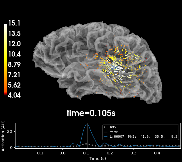
通常，让偶极子具有某种程度的自由方向、但又不过分偏离垂直于皮层的方向，往往能获得最佳结果。mne.minimum_norm.make_inverse_operator() 的 loose 参数允许你指定一个介于 0（固定）和 1（不受限制或“自由”）之间的值，以表示允许方向偏离表面法线的程度。

# Set loose to 0.2, the default value
inv = make_inverse_operator(left_auditory.info, fwd, noise_cov, fixed=False, loose=0.2)
stc = apply_inverse(left_auditory, inv, pick_ori="vector")

# Visualize it at the moment of peak activity.
_, time_max = stc.magnitude().get_peak(hemi="lh")
brain_loose = stc.plot(
    subjects_dir=subjects_dir,
    initial_time=time_max,
    time_unit="s",
    size=(600, 400),
    overlay_alpha=0,
)
mne.viz.set_3d_view(figure=brain_loose, focalpoint=(0.0, 0.0, 50))

Computing inverse operator with 364 channels.
    364 out of 366 channels remain after picking
Selected 364 channels
Creating the depth weighting matrix...
    203 planar channels
    limit = 7262/7498 = 10.020865
    scale = 2.58122e-08 exp = 0.8
Applying loose dipole orientations to surface source spaces: 0.2
Whitening the forward solution.
    Created an SSP operator (subspace dimension = 4)
Computing rank from covariance with rank=None
    Using tolerance 3.3e-13 (2.2e-16 eps * 305 dim * 4.8  max singular value)
    Estimated rank (mag + grad): 302
    MEG: rank 302 computed from 305 data channels with 3 projectors
    Using tolerance 4.7e-14 (2.2e-16 eps * 59 dim * 3.6  max singular value)
    Estimated rank (eeg): 58
    EEG: rank 58 computed from 59 data channels with 1 projector
    Setting small MEG eigenvalues to zero (without PCA)
    Setting small EEG eigenvalues to zero (without PCA)
Creating the source covariance matrix
Adjusting source covariance matrix.
Computing SVD of whitened and weighted lead field matrix.
    largest singular value = 5.49264
    scaling factor to adjust the trace = 1.64e+19 (nchan = 364 nzero = 4)
Preparing the inverse operator for use...
    Scaled noise and source covariance from nave = 1 to nave = 55
    Created the regularized inverter
    Created an SSP operator (subspace dimension = 4)
    Created the whitener using a noise covariance matrix with rank 360 (4 small eigenvalues omitted)
    Computing noise-normalization factors (dSPM)...
[done]
Applying inverse operator to "Left Auditory"...
    Picked 364 channels from the data
    Computing inverse...
    Eigenleads need to be weighted ...
    Computing residual...
    Explained  64.8% variance
    dSPM...
[done]
Using control points [ 4.03844879  4.68532258 15.12541436]

丢弃偶极子方向信息

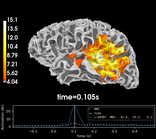
通常，后续数据分析并不需要偶极子方向的信息，而更关心其幅值。mne.minimum_norm.apply_inverse() 函数的 pick_ori 参数允许你指定返回完整向量解（'vector'）、向量幅值（None，默认值），还是仅返回垂直于皮层方向上的活动（'normal'）。

# Only retain vector magnitudes
stc = apply_inverse(left_auditory, inv, pick_ori=None)

# Visualize it at the moment of peak activity
_, time_max = stc.get_peak(hemi="lh")
brain = stc.plot(
    surface="white",
    subjects_dir=subjects_dir,
    initial_time=time_max,
    time_unit="s",
    size=(600, 400),
)
mne.viz.set_3d_view(figure=brain, focalpoint=(0.0, 0.0, 50))

Preparing the inverse operator for use...
    Scaled noise and source covariance from nave = 1 to nave = 55
    Created the regularized inverter
    Created an SSP operator (subspace dimension = 4)
    Created the whitener using a noise covariance matrix with rank 360 (4 small eigenvalues omitted)
    Computing noise-normalization factors (dSPM)...
[done]
Applying inverse operator to "Left Auditory"...
    Picked 364 channels from the data
    Computing inverse...
    Eigenleads need to be weighted ...
    Computing residual...
    Explained  64.8% variance
    Combining the current components...
    dSPM...
[done]
Using control points [ 4.03844879  4.68532258 15.12541436]

参考文献

[1]

Matti S. Hämäläinen, Riitta Hari, Risto J. Ilmoniemi, Jukka Knuutila, and Olli V. Lounasmaa. Magnetoencephalography—theory, instrumentation, and applications to noninvasive studies of the working human brain. Reviews of Modern Physics, 65(2):413–497, 1993. doi:10.1103/RevModPhys.65.413.

[2]

Fa-Hsuan Lin, John W. Belliveau, Anders M. Dale, and Matti S. Hämäläinen. Distributed current estimates using cortical orientation constraints. Human Brain Mapping, 27(1):1–13, 2006. doi:10.1002/hbm.20155.