
说明
转到末尾下载完整示例代码。
可视化源时间过程(STC)#
本教程重点介绍源估计的可视化。
表面源估计#
首先,我们获取诱发数据和源时间过程(STC)的文件路径。
# Authors: The MNE-Python contributors.
# License: BSD-3-Clause
# Copyright the MNE-Python contributors.
import matplotlib.pyplot as plt
import numpy as np

import mne
from mne import read_evokeds
from mne.datasets import fetch_hcp_mmp_parcellation, sample
from mne.minimum_norm import apply_inverse, read_inverse_operator

data_path = sample.data_path()
meg_path = data_path / "MEG" / "sample"
subjects_dir = data_path / "subjects"

fname_evoked = meg_path / "sample_audvis-ave.fif"
fname_stc = meg_path / "sample_audvis-meg"
fetch_hcp_mmp_parcellation(subjects_dir)
然后,我们从文件中读取 STC。
stc = mne.read_source_estimate(fname_stc, subject="sample")
这是一个 SourceEstimate 对象。
print(stc)
<SourceEstimate | 7498 vertices, subject : sample, tmin : 0.0 (ms), tmax : 240.0 (ms), tstep : 10.0 (ms), data shape : (7498, 25), ~791 KiB>
SourceEstimate 对象实际上是表面源估计。MNE 也支持基于体积的源估计,稍后会进一步介绍。
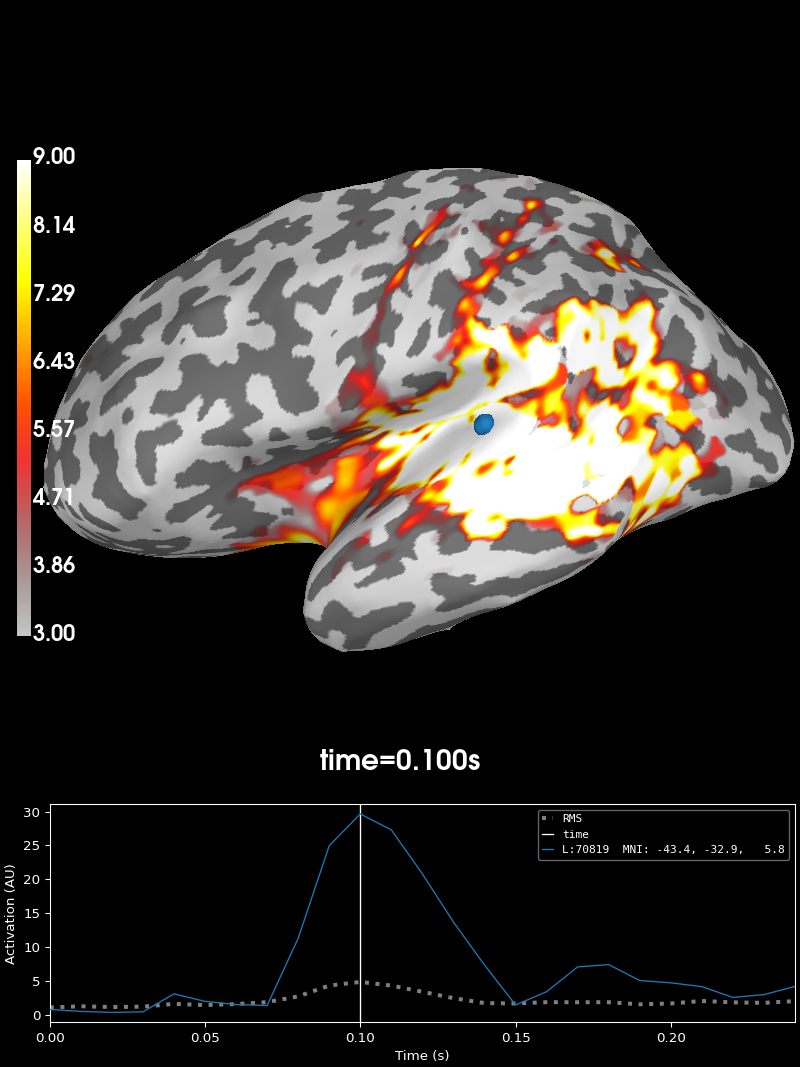
与其他 MNE 对象一样,我们可以使用 stc.plot 绘制源估计。请注意,要使该可视化正常工作,你的机器上必须安装 PyVista。
initial_time = 0.1
brain = stc.plot(
    subjects_dir=subjects_dir,
    initial_time=initial_time,
    clim=dict(kind="value", lims=[3, 6, 9]),
    smoothing_steps=7,
)
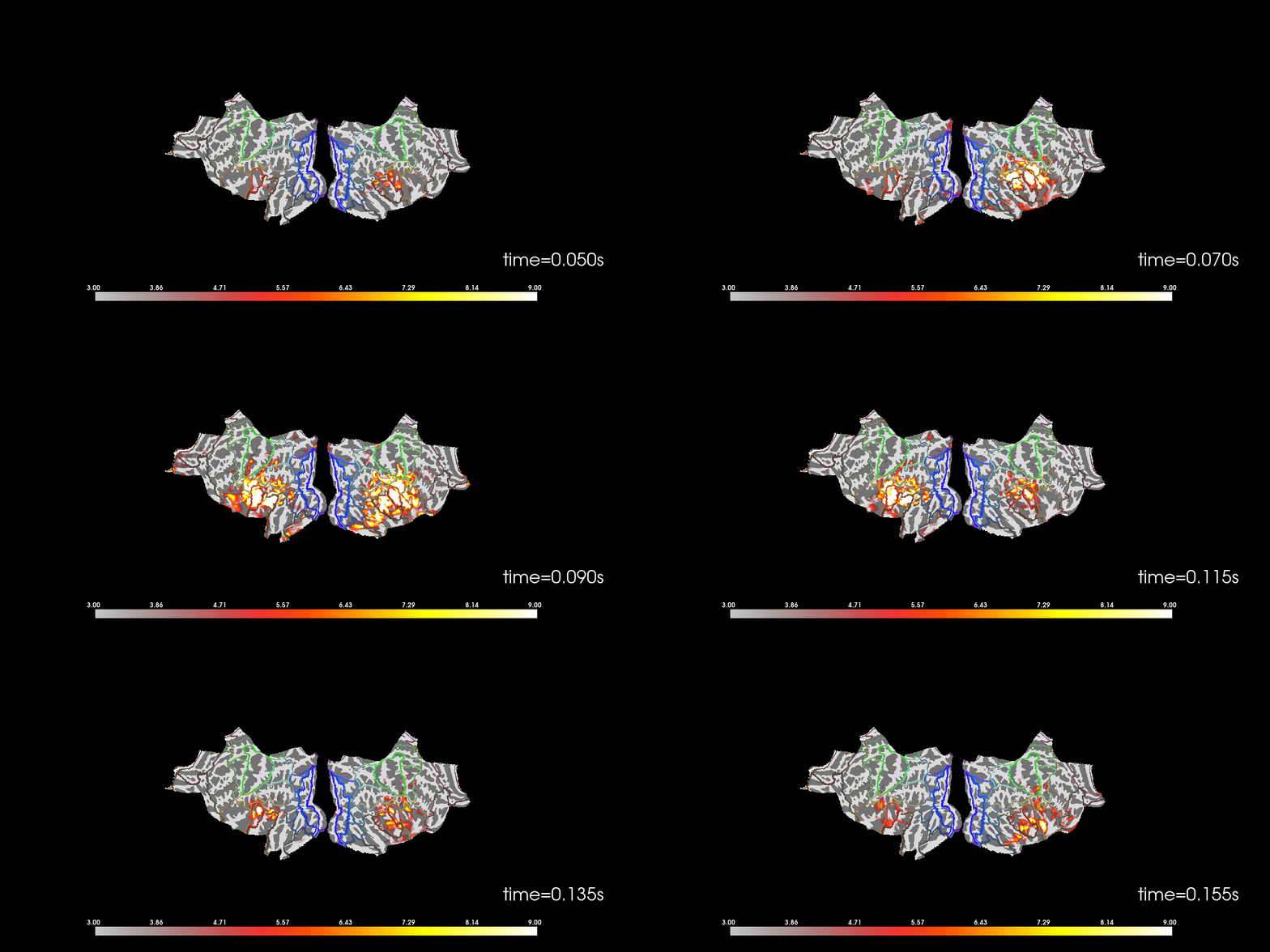
你也可以将其变形到 fsaverage,并使用平展图(flatmap)进行可视化。
stc_fs = mne.compute_source_morph(
    stc, "sample", "fsaverage", subjects_dir, smooth=5, verbose="error"
).apply(stc)
brain = stc_fs.plot(
    subjects_dir=subjects_dir,
    initial_time=initial_time,
    clim=dict(kind="value", lims=[3, 6, 9]),
    surface="flat",
    hemi="both",
    size=(1000, 500),
    smoothing_steps=5,
    time_viewer=False,
    add_data_kwargs=dict(colorbar_kwargs=dict(label_font_size=10)),
)

# to help orient us, let's add a parcellation (red=auditory, green=motor,
# blue=visual)
brain.add_annotation("HCPMMP1_combined", borders=2)

# You can save a movie like the one on our documentation website with:
# brain.save_movie(time_dilation=20, tmin=0.05, tmax=0.16,
#                  interpolation='linear', framerate=10)
Reading labels from parcellation...
   read 23 labels from /home/circleci/mne_data/MNE-sample-data/subjects/fsaverage/label/lh.HCPMMP1_combined.annot
Reading labels from parcellation...
   read 23 labels from /home/circleci/mne_data/MNE-sample-data/subjects/fsaverage/label/rh.HCPMMP1_combined.annot
请注意,这里我们使用了 initial_time=0.1,但也可以通过 time_viewer=True 浏览不同时间点。
体积源估计#
我们还可以可视化体积源估计(用于深部结构)。
让我们加载传感器水平的诱发数据。为简单起见,我们选择 MEG 通道。
evoked = read_evokeds(fname_evoked, condition=0, baseline=(None, 0))
evoked.pick(picks="meg").crop(0.05, 0.15)
# this risks aliasing, but these data are very smooth
evoked.decimate(10, verbose="error")
Reading /home/circleci/mne_data/MNE-sample-data/MEG/sample/sample_audvis-ave.fif ...
    Read a total of 4 projection items:
        PCA-v1 (1 x 10²) active
        PCA-v2 (1 x 10²) active
        PCA-v3 (1 x 10²) active
        Average EEG reference (1 x 60) active
    Found the data of interest:
        t =    -199.80 ...     499.49 ms (Left Auditory)
        0 CTF compensation matrices available
        nave = 55 - aspect type = 100
Projections have already been applied. Setting proj attribute to True.
Applying baseline correction (mode: mean)
然后,我们可以从文件中加载预先计算好的逆算子。
fname_inv = meg_path / "sample_audvis-meg-vol-7-meg-inv.fif"
inv = read_inverse_operator(fname_inv)
src = inv["src"]
mri_head_t = inv["mri_head_t"]
Reading inverse operator decomposition from /home/circleci/mne_data/MNE-sample-data/MEG/sample/sample_audvis-meg-vol-7-meg-inv.fif...
    Reading inverse operator info...
    [done]
    Reading inverse operator decomposition...
    [done]
    305 x 305 full covariance (kind = 1) found.
    Read a total of 4 projection items:
        PCA-v1 (1 x 10²) active
        PCA-v2 (1 x 10²) active
        PCA-v3 (1 x 10²) active
        Average EEG reference (1 x 60) active
    Noise covariance matrix read.
    11271 x 11271 diagonal covariance (kind = 2) found.
    Source covariance matrix read.
    Did not find the desired covariance matrix (kind = 6)
    11271 x 11271 diagonal covariance (kind = 5) found.
    Depth priors read.
    Did not find the desired covariance matrix (kind = 3)
    Reading a source space...
    [done]
    1 source spaces read
    Read a total of 4 projection items:
        PCA-v1 (1 x 10²) active
        PCA-v2 (1 x 10²) active
        PCA-v3 (1 x 10²) active
        Average EEG reference (1 x 60) active
    Source spaces transformed to the inverse solution coordinate frame
源估计是使用逆算子和传感器空间数据计算得到的。
Preparing the inverse operator for use...
    Scaled noise and source covariance from nave = 1 to nave = 55
    Created the regularized inverter
    Created an SSP operator (subspace dimension = 3)
    Created the whitener using a noise covariance matrix with rank 302 (3 small eigenvalues omitted)
    Computing noise-normalization factors (dSPM)...
[done]
Applying inverse operator to "Left Auditory"...
    Picked 305 channels from the data
    Computing inverse...
    Eigenleads need to be weighted ...
    Computing residual...
    Explained  77.1% variance
    Combining the current components...
    dSPM...
[done]
这一次,源时间过程使用了不同的容器(VolSourceEstimate)。
print(stc)
<VolSourceEstimate | 3757 vertices, subject : sample, tmin : 49.94880328959697 (ms), tmax : 149.84640986879091 (ms), tstep : 16.649601096532322 (ms), data shape : (3757, 7), ~235 KiB>
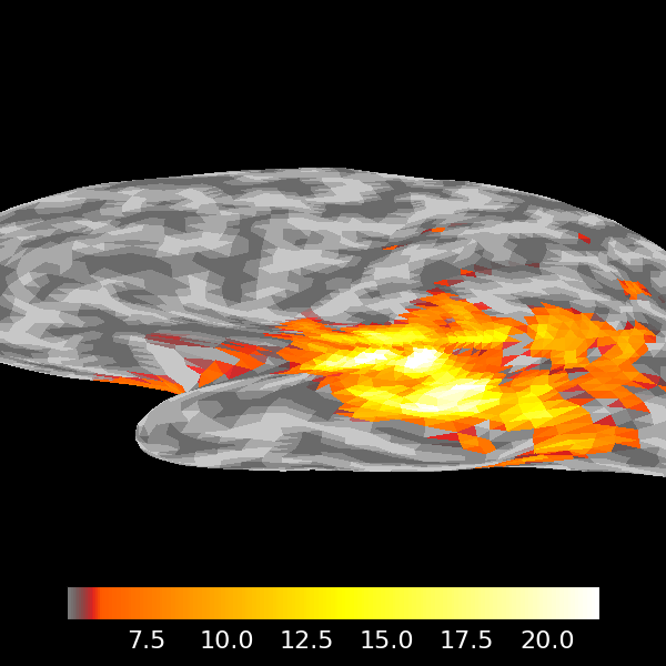
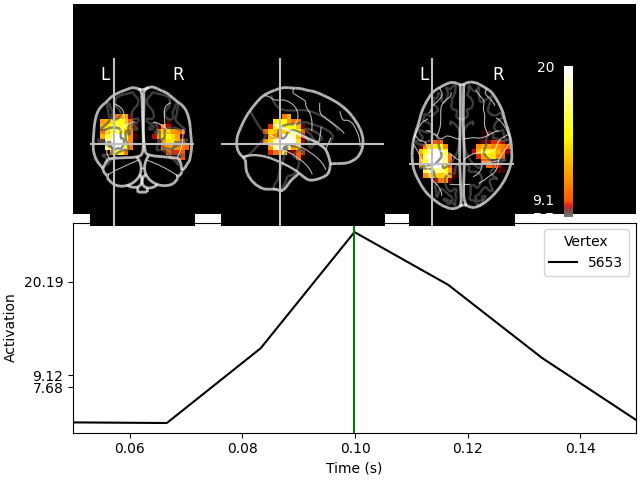
它同样提供了一个便捷的 plot 方法。
stc.plot(src, subject="sample", subjects_dir=subjects_dir)
Showing: t = 0.100 s, (-47.3, -19.0, -6.3) mm, [4, 9, 10] vox, 5653 vertex
Using control points [ 7.67635542  9.11717401 20.19136023]
此可视化需要安装 nilearn。该可视化是交互式的。单击任意解剖切片即可查看时间序列。单击任意时间点将显示相应的解剖图。
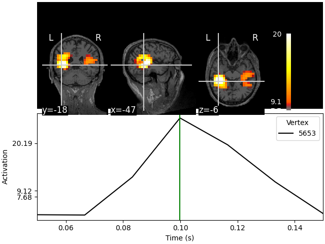
我们还可以在玻璃脑(glass brain)上可视化源估计。与之前的可视化不同,玻璃脑并不显示单个切片,而是显示大脑像玻璃一样透明时我们所看到的效果,并使用了最大强度投影(MIP):
stc.plot(src, subject="sample", subjects_dir=subjects_dir, mode="glass_brain")
Transforming subject RAS (non-zero origin) -> MNI Talairach
    1.022485 -0.008449 -0.036217       5.60 mm
    0.071071 0.914866 0.406098     -19.82 mm
    0.008756 -0.433700 1.028119      -1.55 mm
    0.000000 0.000000 0.000000       1.00

Showing: t = 0.100 s, (-42.4, -43.1, -0.2) mm, [4, 9, 10] vox, 5653 vertex
Using control points [ 7.67635542  9.11717401 20.19136023]
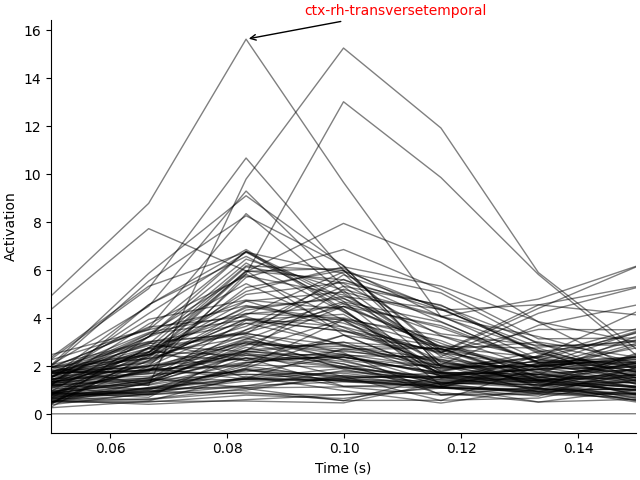
你还可以使用体积图谱提取标签时间过程。这里我们将使用内置的 aparc+aseg.mgz:
fname_aseg = subjects_dir / "sample" / "mri" / "aparc+aseg.mgz"
label_names = mne.get_volume_labels_from_aseg(fname_aseg)
label_tc = stc.extract_label_time_course(fname_aseg, src=src)

lidx, tidx = np.unravel_index(np.argmax(label_tc), label_tc.shape)
fig, ax = plt.subplots(1, layout="constrained")
ax.plot(stc.times, label_tc.T, "k", lw=1.0, alpha=0.5)
xy = np.array([stc.times[tidx], label_tc[lidx, tidx]])
xytext = xy + [0.01, 1]
ax.annotate(label_names[lidx], xy, xytext, arrowprops=dict(arrowstyle="->"), color="r")
ax.set(xlim=stc.times[[0, -1]], xlabel="Time (s)", ylabel="Activation")
for key in ("right", "top"):
    ax.spines[key].set_visible(False)
Reading atlas /home/circleci/mne_data/MNE-sample-data/subjects/sample/mri/aparc+aseg.mgz
114/114 atlas regions had at least one vertex in the source space
Extracting time courses for 114 labels (mode: mean)
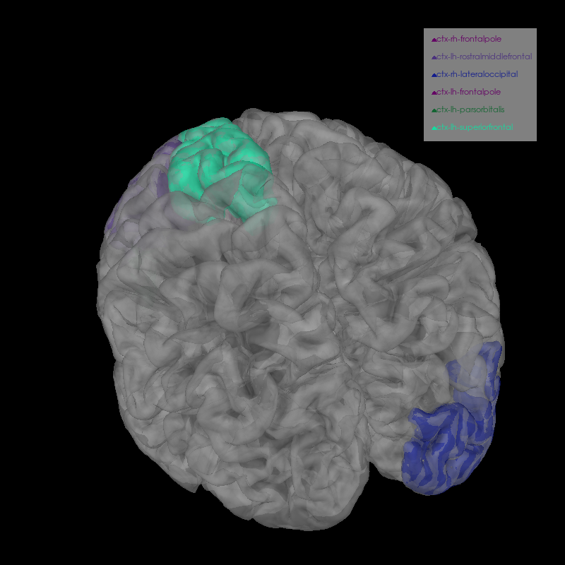
我们可以绘制时间过程中激活最强的几个标签,以更精细地查看激活的解剖位置。
labels = [
    label_names[idx]
    for idx in np.argsort(label_tc.max(axis=1))[:7]
    if "unknown" not in label_names[idx].lower()
]  # remove catch-all
brain = mne.viz.Brain(
    "sample",
    hemi="both",
    surf="pial",
    alpha=0.5,
    cortex="low_contrast",
    subjects_dir=subjects_dir,
)
brain.add_volume_labels(aseg="aparc+aseg", labels=labels)
brain.show_view(azimuth=250, elevation=40, distance=400)
Smoothing by a factor of 0.9
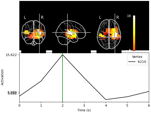
我们还可以将这些标签时间过程投影回其原始位置,并查看绘图是如何被平滑的:
stc_back = mne.labels_to_stc(fname_aseg, label_tc, src=src)
stc_back.plot(src, subjects_dir=subjects_dir, mode="glass_brain")
Reading atlas /home/circleci/mne_data/MNE-sample-data/subjects/sample/mri/aparc+aseg.mgz
114/114 atlas regions had at least one vertex in the source space
Extracting time courses for 114 labels (mode: mean)
Transforming subject RAS (non-zero origin) -> MNI Talairach
    1.022485 -0.008449 -0.036217       5.60 mm
    0.071071 0.914866 0.406098     -19.82 mm
    0.008756 -0.433700 1.028119      -1.55 mm
    0.000000 0.000000 0.000000       1.00

Showing: t = 2.000 s, (36.1, -34.8, 7.7) mm, [15, 9, 11] vox, 6210 vertex
Using control points [ 5.69834054  5.98871778 15.62206532]
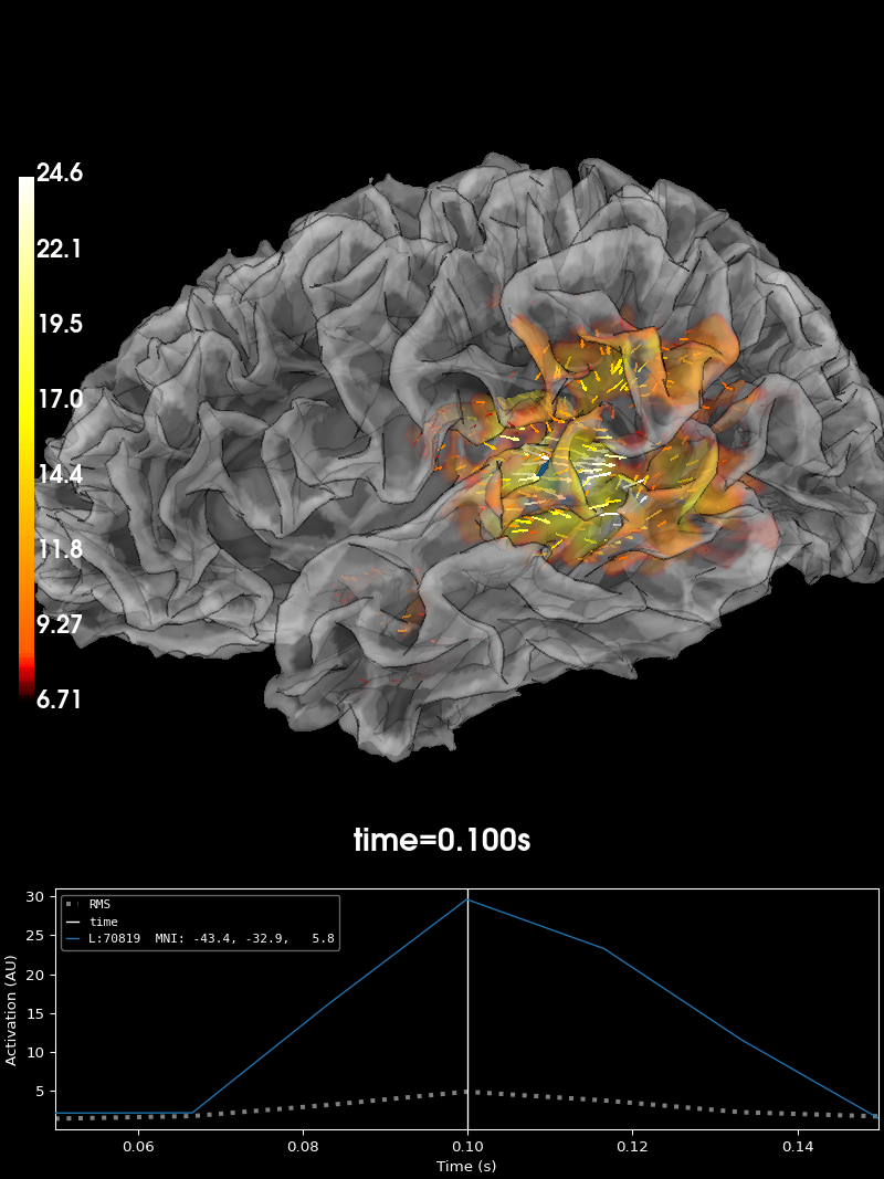
矢量源估计#
如果我们在 apply_inverse 中选择使用 pick_ori='vector'
fname_inv = data_path / "MEG" / "sample" / "sample_audvis-meg-oct-6-meg-inv.fif"
inv = read_inverse_operator(fname_inv)
stc = apply_inverse(evoked, inv, lambda2, "dSPM", pick_ori="vector")
brain = stc.plot(
    subject="sample",
    subjects_dir=subjects_dir,
    initial_time=initial_time,
    brain_kwargs=dict(silhouette=True),
    smoothing_steps=7,
)
Reading inverse operator decomposition from /home/circleci/mne_data/MNE-sample-data/MEG/sample/sample_audvis-meg-oct-6-meg-inv.fif...
    Reading inverse operator info...
    [done]
    Reading inverse operator decomposition...
    [done]
    305 x 305 full covariance (kind = 1) found.
    Read a total of 4 projection items:
        PCA-v1 (1 x 10²) active
        PCA-v2 (1 x 10²) active
        PCA-v3 (1 x 10²) active
        Average EEG reference (1 x 60) active
    Noise covariance matrix read.
    22494 x 22494 diagonal covariance (kind = 2) found.
    Source covariance matrix read.
    22494 x 22494 diagonal covariance (kind = 6) found.
    Orientation priors read.
    22494 x 22494 diagonal covariance (kind = 5) found.
    Depth priors read.
    Did not find the desired covariance matrix (kind = 3)
    Reading a source space...
    Computing patch statistics...
    Patch information added...
    Distance information added...
    [done]
    Reading a source space...
    Computing patch statistics...
    Patch information added...
    Distance information added...
    [done]
    2 source spaces read
    Read a total of 4 projection items:
        PCA-v1 (1 x 10²) active
        PCA-v2 (1 x 10²) active
        PCA-v3 (1 x 10²) active
        Average EEG reference (1 x 60) active
    Source spaces transformed to the inverse solution coordinate frame
Preparing the inverse operator for use...
    Scaled noise and source covariance from nave = 1 to nave = 55
    Created the regularized inverter
    Created an SSP operator (subspace dimension = 3)
    Created the whitener using a noise covariance matrix with rank 302 (3 small eigenvalues omitted)
    Computing noise-normalization factors (dSPM)...
[done]
Applying inverse operator to "Left Auditory"...
    Picked 305 channels from the data
    Computing inverse...
    Eigenleads need to be weighted ...
    Computing residual...
    Explained  77.5% variance
    dSPM...
[done]
Using control points [ 6.70708526  8.36619556 24.64056812]
    Triangle neighbors and vertex normals...
Loading geometry from /home/circleci/mne_data/MNE-sample-data/subjects/sample/surf/lh.sphere...
Setting up the triangulation for the decimated surface...
偶极子拟合#
为了计算偶极子拟合,我们需要加载噪声协方差、BEM 解以及配准变换文件。请注意,对于其他方法,这些文件已经用于生成逆算子。
fname_cov = meg_path / "sample_audvis-cov.fif"
fname_bem = subjects_dir / "sample" / "bem" / "sample-5120-bem-sol.fif"
fname_trans = meg_path / "sample_audvis_raw-trans.fif"
偶极子是针对每个时间点独立拟合的,因此让我们裁剪时间序列,以便可视化感兴趣时间点的偶极子拟合。
evoked.crop(0.1, 0.1)
dip = mne.fit_dipole(evoked, fname_cov, fname_bem, fname_trans)[0]
BEM               : PosixPath('/home/circleci/mne_data/MNE-sample-data/subjects/sample/bem/sample-5120-bem-sol.fif')
MRI transform     : /home/circleci/mne_data/MNE-sample-data/MEG/sample/sample_audvis_raw-trans.fif
Head origin       :   -4.2   19.3   65.3 mm rad =   72.3 mm.
Guess grid        :   20.0 mm
Guess mindist     :    5.0 mm
Guess exclude     :   20.0 mm
Using normal MEG coil definitions.
Noise covariance  : /home/circleci/mne_data/MNE-sample-data/MEG/sample/sample_audvis-cov.fif

Coordinate transformation: MRI (surface RAS) -> head
    0.999310 0.009985 -0.035787      -3.17 mm
    0.012759 0.812405 0.582954       6.86 mm
    0.034894 -0.583008 0.811716      28.88 mm
    0.000000 0.000000 0.000000       1.00
Coordinate transformation: MEG device -> head
    0.991420 -0.039936 -0.124467      -6.13 mm
    0.060661 0.984012 0.167456       0.06 mm
    0.115790 -0.173570 0.977991      64.74 mm
    0.000000 0.000000 0.000000       1.00
1 bad channels total
Read 305 MEG channels from info
105 coil definitions read
Coordinate transformation: MEG device -> head
    0.991420 -0.039936 -0.124467      -6.13 mm
    0.060661 0.984012 0.167456       0.06 mm
    0.115790 -0.173570 0.977991      64.74 mm
    0.000000 0.000000 0.000000       1.00
MEG coil definitions created in head coordinates.
Decomposing the sensor noise covariance matrix...
    Created an SSP operator (subspace dimension = 3)
Computing rank from covariance with rank=None
    Using tolerance 3.3e-13 (2.2e-16 eps * 305 dim * 4.8  max singular value)
    Estimated rank (mag + grad): 302
    MEG: rank 302 computed from 305 data channels with 3 projectors
    Setting small MEG eigenvalues to zero (without PCA)
    Created the whitener using a noise covariance matrix with rank 302 (3 small eigenvalues omitted)

---- Computing the forward solution for the guesses...
Guess surface (inner skull) is in MRI (surface RAS) coordinates
Filtering (grid =     20 mm)...
Surface CM = (   0.7  -10.0   44.3) mm
Surface fits inside a sphere with radius   91.8 mm
Surface extent:
    x =  -66.7 ...   68.8 mm
    y =  -88.0 ...   79.0 mm
    z =  -44.5 ...  105.8 mm
Grid extent:
    x =  -80.0 ...   80.0 mm
    y = -100.0 ...   80.0 mm
    z =  -60.0 ...  120.0 mm
900 sources before omitting any.
396 sources after omitting infeasible sources not within 20.0 - 91.8 mm.
Source spaces are in MRI coordinates.
Checking that the sources are inside the surface and at least    5.0 mm away (will take a few...)
Checking surface interior status for 396 points...
    Found  42/396 points inside  an interior sphere of radius   43.6 mm
    Found   0/396 points outside an exterior sphere of radius   91.8 mm
    Found 186/354 points outside using surface Qhull
    Found   9/168 points outside using solid angles
    Total 201/396 points inside the surface
Interior check completed in 15.5 ms
    195 source space points omitted because they are outside the inner skull surface.
    45 source space points omitted because of the    5.0-mm distance limit.
156 sources remaining after excluding the sources outside the surface and less than    5.0 mm inside.
Go through all guess source locations...
[done 156 sources]
---- Fitted :    99.9 ms, distance to inner skull : 7.6207 mm
Projections have already been applied. Setting proj attribute to True.
1 time points fitted
最后,我们可以可视化偶极子。
dip.plot_locations(fname_trans, "sample", subjects_dir)
脚本总运行时间:(0 分钟 40.324 秒)