
说明
转到末尾下载完整示例代码。
基于 MRI 电极位置的 EEG 源定位#
本教程说明当电极位于 MRI 体素坐标时,如何根据 EEG 数据计算前向算子。
# Authors: Eric Larson <larson.eric.d@gmail.com>
#
# License: BSD-3-Clause
# Copyright the MNE-Python contributors.
import nibabel
import numpy as np
from nilearn.plotting import plot_glass_brain

import mne
from mne.channels import compute_native_head_t, read_custom_montage
from mne.viz import plot_alignment
前提条件#
为此,我们假设你已具备:
原始 EEG 数据
使用 FreeSurfer 重建的被试 MRI
合适的边界元模型(BEM)
合适的源空间(src)
你的 EEG 电极位置已转换为 FreeSurfer 表面 RAS 坐标,并以
mne.channels.read_custom_montage()支持的某种格式存储
下面为示例数据集设置这些文件的路径,其中包括一个修改过的示例 MRI(显示电极位置)以及一个与 MRI 坐标中这些点对应的 .elc 文件(这些点是合成的,因此作为 misc 数据集的一部分存储)。
data_path = mne.datasets.sample.data_path()
subjects_dir = data_path / "subjects"
fname_raw = data_path / "MEG" / "sample" / "sample_audvis_raw.fif"
bem_dir = subjects_dir / "sample" / "bem"
fname_bem = bem_dir / "sample-5120-5120-5120-bem-sol.fif"
fname_src = bem_dir / "sample-oct-6-src.fif"

misc_path = mne.datasets.misc.data_path()
fname_T1_electrodes = misc_path / "sample_eeg_mri" / "T1_electrodes.mgz"
fname_mon = misc_path / "sample_eeg_mri" / "sample_mri_montage.elc"
可视化 MRI#
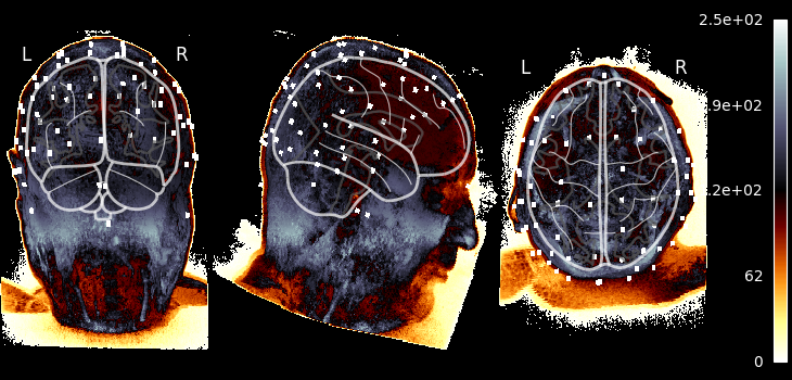
让我们取出带 EEG 电极位置的 MRI,调整仿射矩阵以将数据放入 MNI 空间,并使用 nilearn.plotting.plot_glass_brain() 绘图,该函数执行最大强度投影(便于看到那些模拟电极)。此绘图函数要求数据位于 MNI 空间。由于 img.affine 给出体素到世界(RAS)的映射,若对其应用 RAS 到 MNI 的变换,它就变成我们所需的体素到 MNI 变换。因此我们创建一个位于 MNI 坐标的“新”MRI 图像并绘图:
img = nibabel.load(fname_T1_electrodes)  # original subject MRI w/EEG
ras_mni_t = mne.transforms.read_ras_mni_t("sample", subjects_dir)  # from FS
mni_affine = np.dot(ras_mni_t["trans"], img.affine)  # vox->ras->MNI
img_mni = nibabel.Nifti1Image(img.dataobj, mni_affine)  # now in MNI coords!
plot_glass_brain(
    img_mni,
    cmap="hot_black_bone",
    threshold=0.0,
    black_bg=True,
    resampling_interpolation="nearest",
    colorbar=True,
)
将 MRI 体素中的 EEG 电极位置转换到头部(及 MRI 表面 RAS)坐标#
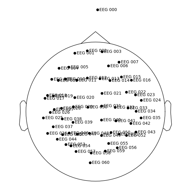
我们使用 mne.channels.read_custom_montage() 加载 DigMontage,并注意我们将位置存储在 FreeSurfer 表面 RAS(MRI)坐标中。
What if my electrodes are in MRI voxels?
如果你拥有 MRI 体素坐标,可以使用 FreeSurfer 在重建过程中计算的变换,将其转换为 FreeSurfer 表面 RAS(在 MNE 中称为 mri)坐标。nibabel 将该变换称为 vox2ras_tkr,并以毫米为单位,因此我们可以加载它、转换为米,然后应用:
你也可以在 Freeview 或 tkmedit 中查看这些点,以验证它们是否正确(或手动将体素转换为 MRI 坐标)。
dig_montage = read_custom_montage(
    fname_mon,
    head_size=None,
    coord_frame="mri",
    verbose="error",  # because it contains a duplicate point
)
dig_montage.plot()
然后,我们可以从该对象获取从 MRI 坐标系(这些点定义所在的坐标系)到头部坐标系的变换。
trans = compute_native_head_t(dig_montage)
print(trans)  # should be mri->head, as the "native" space here is MRI
<Transform | MRI (surface RAS)->head>
[[ 0.99930957  0.00998471 -0.03578661 -0.00316747]
 [ 0.01275917  0.81240435  0.58295487  0.00685511]
 [ 0.03489383 -0.58300899  0.81171605  0.02888406]
 [ 0.          0.          0.          1.        ]]
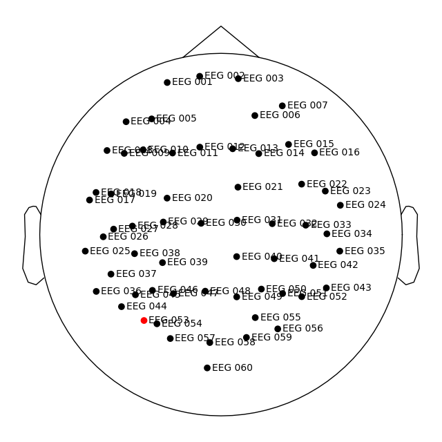
我们将此数字化信息应用到数据集,并在此过程中自动将位置转换到头部坐标系,如 plot_sensors() 所示。
raw = mne.io.read_raw_fif(fname_raw)
raw.pick(picks=["eeg", "stim"]).load_data()
raw.set_montage(dig_montage)
raw.plot_sensors(show_names=True)
Opening raw data file /home/circleci/mne_data/MNE-sample-data/MEG/sample/sample_audvis_raw.fif...
    Read a total of 3 projection items:
        PCA-v1 (1 x 10²)  idle
        PCA-v2 (1 x 10²)  idle
        PCA-v3 (1 x 10²)  idle
    Range : 25800 ... 192599 =     42.956 ...   320.670 secs
Ready.
Reading 0 ... 166799  =      0.000 ...   277.714 secs...
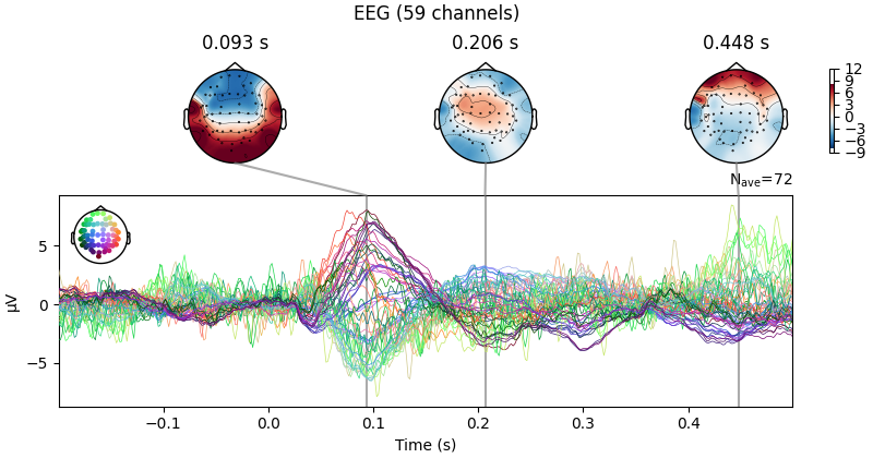
现在我们可以执行标准的传感器空间操作,例如绘制诱发数据的联合图。
raw.set_eeg_reference(projection=True)
events = mne.find_events(raw)
epochs = mne.Epochs(raw, events)
cov = mne.compute_covariance(epochs, tmax=0.0)
evoked = epochs["1"].average()  # trigger 1 in auditory/left
evoked.plot_joint()
EEG channel type selected for re-referencing
Adding average EEG reference projection.
1 projection items deactivated
Average reference projection was added, but has not been applied yet. Use the apply_proj method to apply it.
Finding events on: STI 014
320 events found on stim channel STI 014
Event IDs: [ 1  2  3  4  5 32]
Not setting metadata
320 matching events found
Setting baseline interval to [-0.19979521315838786, 0.0] s
Applying baseline correction (mode: mean)
Created an SSP operator (subspace dimension = 1)
1 projection items activated
Using data from preloaded Raw for 72 events and 421 original time points ...
0 bad epochs dropped
Using data from preloaded Raw for 73 events and 421 original time points ...
0 bad epochs dropped
Using data from preloaded Raw for 73 events and 421 original time points ...
0 bad epochs dropped
Using data from preloaded Raw for 71 events and 421 original time points ...
0 bad epochs dropped
Using data from preloaded Raw for 15 events and 421 original time points ...
0 bad epochs dropped
Using data from preloaded Raw for 16 events and 421 original time points ...
0 bad epochs dropped
    Created an SSP operator (subspace dimension = 1)
    Setting small EEG eigenvalues to zero (without PCA)
Reducing data rank from 59 -> 58
Estimating covariance using EMPIRICAL
Done.
Number of samples used : 38720
[done]
Projections have already been applied. Setting proj attribute to True.
获取源估计#
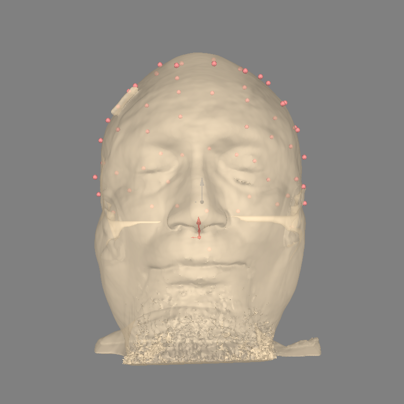
现在我们已经具备计算前向解所需的全部组件,但首先应检查所有内容是否对齐良好:
fig = plot_alignment(
    evoked.info,
    trans=trans,
    show_axes=True,
    surfaces="head-dense",
    subject="sample",
    subjects_dir=subjects_dir,
)
Using lh.seghead for head surface.
Channel types:: eeg: 59
现在我们可以实际计算前向解:
fwd = mne.make_forward_solution(
    evoked.info, trans=trans, src=fname_src, bem=fname_bem, verbose=True
)
Source space          : /home/circleci/mne_data/MNE-sample-data/subjects/sample/bem/sample-oct-6-src.fif
MRI -> head transform : instance of Transform
Measurement data      : instance of Info
Conductor model   : /home/circleci/mne_data/MNE-sample-data/subjects/sample/bem/sample-5120-5120-5120-bem-sol.fif
Accurate field computations
Do computations in head coordinates
Free source orientations

Reading /home/circleci/mne_data/MNE-sample-data/subjects/sample/bem/sample-oct-6-src.fif...
Read 2 source spaces a total of 8196 active source locations

Coordinate transformation: MRI (surface RAS) -> head
    0.999310 0.009985 -0.035787      -3.17 mm
    0.012759 0.812404 0.582955       6.86 mm
    0.034894 -0.583009 0.811716      28.88 mm
    0.000000 0.000000 0.000000       1.00

Read  60 EEG channels from info
Head coordinate coil definitions created.
Source spaces are now in head coordinates.

Setting up the BEM model using /home/circleci/mne_data/MNE-sample-data/subjects/sample/bem/sample-5120-5120-5120-bem-sol.fif...

Loading surfaces...

Loading the solution matrix...

Three-layer model surfaces loaded.
Loaded linear collocation BEM solution from /home/circleci/mne_data/MNE-sample-data/subjects/sample/bem/sample-5120-5120-5120-bem-sol.fif
Employing the head->MRI coordinate transform with the BEM model.
BEM model sample-5120-5120-5120-bem-sol.fif is now set up


Source spaces are in head coordinates.
Checking that the sources are inside the surface (will take a few...)
Checking surface interior status for 4098 points...
    Found  846/4098 points inside  an interior sphere of radius   43.6 mm
    Found    0/4098 points outside an exterior sphere of radius   91.8 mm
    Found    2/3252 points outside using surface Qhull
    Found    0/3250 points outside using solid angles
    Total 4096/4098 points inside the surface
Interior check completed in 221.4 ms
    2 source space points omitted because they are outside the inner skull surface.
    Computing patch statistics...
    Patch information added...
Checking surface interior status for 4098 points...
    Found  875/4098 points inside  an interior sphere of radius   43.6 mm
    Found    0/4098 points outside an exterior sphere of radius   91.8 mm
    Found    0/3223 points outside using surface Qhull
    Found    1/3223 point  outside using solid angles
    Total 4097/4098 points inside the surface
Interior check completed in 214.6 ms
    1 source space point omitted because it is outside the inner skull surface.
    Computing patch statistics...
    Patch information added...
Setting up for EEG...
Computing EEG at 8193 source locations (free orientations)...

Finished.
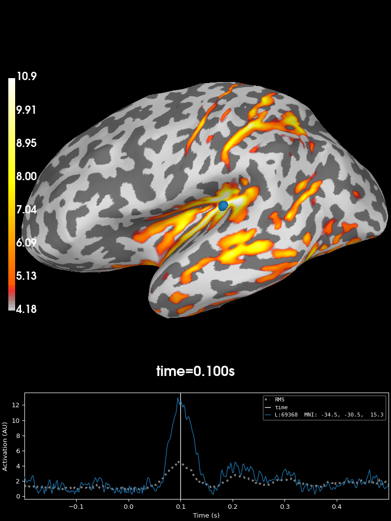
最后,我们计算逆算子并应用它:
inv = mne.minimum_norm.make_inverse_operator(evoked.info, fwd, cov, verbose=True)
stc = mne.minimum_norm.apply_inverse(evoked, inv)
brain = stc.plot(subjects_dir=subjects_dir, initial_time=0.1)
Converting forward solution to surface orientation
    Average patch normals will be employed in the rotation to the local surface coordinates....
    Converting to surface-based source orientations...
    [done]
info["bads"] and noise_cov["bads"] do not match, excluding bad channels from both
Computing inverse operator with 59 channels.
    59 out of 60 channels remain after picking
Selected 59 channels
Creating the depth weighting matrix...
    59 EEG channels
    limit = 8192/8193 = 10.040598
    scale = 157084 exp = 0.8
Applying loose dipole orientations to surface source spaces: 0.2
Whitening the forward solution.
    Created an SSP operator (subspace dimension = 1)
Computing rank from covariance with rank=None
    Using tolerance 1.2e-13 (2.2e-16 eps * 59 dim * 9  max singular value)
    Estimated rank (eeg): 58
    EEG: rank 58 computed from 59 data channels with 1 projector
    Setting small EEG eigenvalues to zero (without PCA)
Creating the source covariance matrix
Adjusting source covariance matrix.
Computing SVD of whitened and weighted lead field matrix.
    largest singular value = 2.86184
    scaling factor to adjust the trace = 3.24877e+19 (nchan = 59 nzero = 1)
Preparing the inverse operator for use...
    Scaled noise and source covariance from nave = 1 to nave = 72
    Created the regularized inverter
    Created an SSP operator (subspace dimension = 1)
    Created the whitener using a noise covariance matrix with rank 58 (1 small eigenvalues omitted)
    Computing noise-normalization factors (dSPM)...
[done]
Applying inverse operator to "1"...
    Picked 59 channels from the data
    Computing inverse...
    Eigenleads need to be weighted ...
    Computing residual...
    Explained  85.0% variance
    Combining the current components...
    dSPM...
[done]
Using control points [ 4.17591891  4.939572   10.86348066]
脚本总运行时间:(0 分钟 13.469 秒)