
说明
转到末尾下载完整示例代码。
光泵磁力仪(OPM)MEG 数据预处理#
本教程介绍针对 OPM MEG 数据的特定预处理步骤。OPM 采用与传统 SQUID MEG 系统不同的传感技术,因此在分析上存在若干重要差异:
它们对直流磁场敏感
由于传感器可灵活放置,传感器布局可能因被试和记录场次而异
设备通常并非固定安装,因此传感器相对于房间的位置(以及所穿过的直流场)会随时间变化
下面我们通过处理 UCL OPM 听觉数据集 [ 1 ] 来讨论其中的一些考量。
# Authors: The MNE-Python contributors.
# License: BSD-3-Clause
# Copyright the MNE-Python contributors.
import matplotlib.pyplot as plt
import nibabel as nib
import numpy as np

import mne

subject = "sub-002"
data_path = mne.datasets.ucl_opm_auditory.data_path()
opm_file = (
    data_path / subject / "ses-001" / "meg" / "sub-002_ses-001_task-aef_run-001_meg.bin"
)
subjects_dir = data_path / "derivatives" / "freesurfer" / "subjects"

# For now we are going to assume the device and head coordinate frames are
# identical (even though this is incorrect), so we pass verbose='error'
raw = mne.io.read_raw_fil(opm_file, verbose="error")
raw.crop(120, 210).load_data()  # crop for speed
Reading 0 ... 540000 = 0.000 ... 90.000 secs...
检查原始数据#
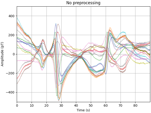
首先观察原始数据,可以看到 1 Hz 以下频段存在大幅波动。在某些情况下,单个通道在整个实验过程中报告的磁场范围可达 600 pT。
picks = mne.pick_types(raw.info, meg=True)

amp_scale = 1e12  # T->pT
stop = len(raw.times) - 300
step = 300
data_ds, time_ds = raw[picks[::5], :stop]
data_ds, time_ds = data_ds[:, ::step] * amp_scale, time_ds[::step]

fig, ax = plt.subplots(layout="constrained")
plot_kwargs = dict(lw=1, alpha=0.5)
ax.plot(time_ds, data_ds.T - np.mean(data_ds, axis=1), **plot_kwargs)
ax.grid(True)
set_kwargs = dict(
    ylim=(-500, 500), xlim=time_ds[[0, -1]], xlabel="Time (s)", ylabel="Amplitude (pT)"
)
ax.set(title="No preprocessing", **set_kwargs)
去噪:基于参考传感器回归#
降低数据中低频漂移最简单的方法是使用一组远离头皮的参考传感器,它们只采集房间内的环境磁场。该方法的优点是不需要预先知道传感器的位置;但它假设参考传感器所受到的干扰与头皮记录相同。
在当前数据集上实现这一点需要先做一些清理工作。有一组以 Flux 开头的通道不包含任何环境数据,需要将它们标记为坏道;另一个通道 G2-17-TAN 也将标记为坏道。
目前我们只关心去除 5 Hz 以下的伪迹,因此在回归之前先对该数据集中质量良好的参考通道进行低通滤波。
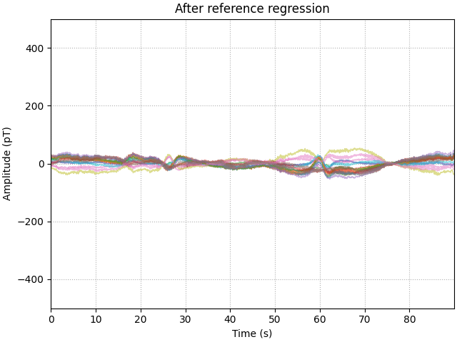
观察处理后的数据可以发现,低频漂移已大幅降低,但仍有一些时段漂移未被完全去除。可能的原因是干扰的空间分布是动态变化的,因此在整个实验上只做一次回归并不是最有效的方法。
# set flux channels to bad
bad_picks = mne.pick_channels_regexp(raw.ch_names, regexp="Flux.")
raw.info["bads"].extend([raw.ch_names[ii] for ii in bad_picks])
raw.info["bads"].extend(["G2-17-TAN"])

# compute the PSD for later using 1 Hz resolution
psd_kwargs = dict(fmax=20, n_fft=int(round(raw.info["sfreq"])))
psd_pre = raw.compute_psd(**psd_kwargs)

# filter and regress
raw.filter(None, 5, picks="ref_meg")
regress = mne.preprocessing.EOGRegression(picks, picks_artifact="ref_meg")
regress.fit(raw)
regress.apply(raw, copy=False)

# plot
data_ds, _ = raw[picks[::5], :stop]
data_ds = data_ds[:, ::step] * amp_scale

fig, ax = plt.subplots(layout="constrained")
ax.plot(time_ds, data_ds.T - np.mean(data_ds, axis=1), **plot_kwargs)
ax.grid(True, ls=":")
ax.set(title="After reference regression", **set_kwargs)

# compute the psd of the regressed data
psd_post_reg = raw.compute_psd(**psd_kwargs)
Effective window size : 1.000 (s)
Filtering a subset of channels. The highpass and lowpass values in the measurement info will not be updated.
Filtering raw data in 1 contiguous segment
Setting up low-pass filter at 5 Hz

FIR filter parameters
---------------------
Designing a one-pass, zero-phase, non-causal lowpass filter:
- Windowed time-domain design (firwin) method
- Hamming window with 0.0194 passband ripple and 53 dB stopband attenuation
- Upper passband edge: 5.00 Hz
- Upper transition bandwidth: 2.00 Hz (-6 dB cutoff frequency: 6.00 Hz)
- Filter length: 9901 samples (1.650 s)

No projector specified for this dataset. Please consider the method self.add_proj.
No projector specified for this dataset. Please consider the method self.add_proj.
Effective window size : 1.000 (s)
去噪:基于均匀场校正的回归#
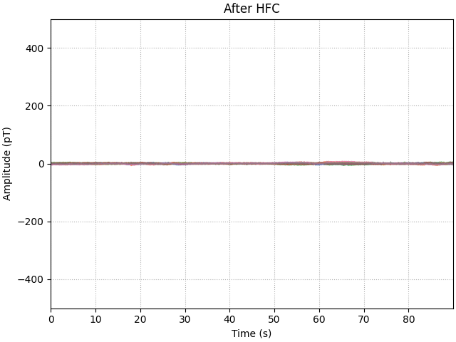
参考通道回归只是一个起点,但在此情况下它假设参考传感器与头部某个传感器之间的关系保持恒定。当参考传感器不动而被试在移动时,这种假设就不那么准确了。另一种方法是均匀场校正(Homogeneous Field Correction,HFC),它只要求头盔上的传感器彼此之间保持相对静止——在设计良好的刚性头盔中正是如此。
# include gradients by setting order to 2, set to 1 for homogeneous components
projs = mne.preprocessing.compute_proj_hfc(raw.info, order=2)
raw.add_proj(projs).apply_proj(verbose="error")

# plot
data_ds, _ = raw[picks[::5], :stop]
data_ds = data_ds[:, ::step] * amp_scale

fig, ax = plt.subplots(layout="constrained")
ax.plot(time_ds, data_ds.T - np.mean(data_ds, axis=1), **plot_kwargs)
ax.grid(True, ls=":")
ax.set(title="After HFC", **set_kwargs)

# compute the psd of the regressed data
psd_post_hfc = raw.compute_psd(**psd_kwargs)
8 projection items deactivated
Effective window size : 1.000 (s)
比较去噪方法#
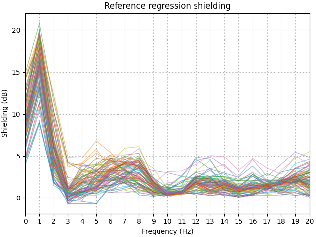
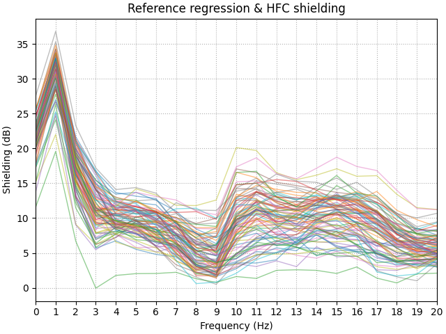
不同的去噪方法在频谱不同部分的性能各异。评估某一步去噪效果的一种方法是计算处理前后数据集的功率谱。我们将用称为屏蔽因子(shielding factor)的指标来概括这些数值:正的屏蔽因子表示功率降低,负值则表示功率增加。
可以看到,参考回归在约 2 Hz 以下能很好地降低低频漂移,屏蔽效果达 20 dB;但由于参考信号在 5 Hz 处被低通滤波,其效果在此之后迅速衰减。我们还能看到该方法在 3 Hz 处引入了额外的干扰。
HFC 进一步改善了低频屏蔽效果(最高达 32 dB)。此外,该方法并不针对特定频率,因此可以观察到宽带干扰的降低。
shielding = 10 * np.log10(psd_pre[:] / psd_post_reg[:])

fig, ax = plt.subplots(layout="constrained")
ax.plot(psd_post_reg.freqs, shielding.T, **plot_kwargs)
ax.grid(True, ls=":")
ax.set(xticks=psd_post_reg.freqs)
ax.set(
    xlim=(0, 20),
    title="Reference regression shielding",
    xlabel="Frequency (Hz)",
    ylabel="Shielding (dB)",
)


shielding = 10 * np.log10(psd_pre[:] / psd_post_hfc[:])

fig, ax = plt.subplots(layout="constrained")
ax.plot(psd_post_hfc.freqs, shielding.T, **plot_kwargs)
ax.grid(True, ls=":")
ax.set(xticks=psd_post_hfc.freqs)
ax.set(
    xlim=(0, 20),
    title="Reference regression & HFC shielding",
    xlabel="Frequency (Hz)",
    ylabel="Shielding (dB)",
)
滤波去除干扰信号#
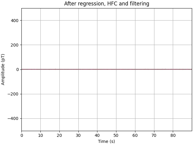
在回归掉大部分高幅低频干扰之后,我们现在可以着眼于滤除残余的干扰信号。之所以在回归之后(而不是之前)进行滤波,是为了尽量减少去除这类高幅干扰时产生的滤波伪迹(相对于我们感兴趣的神经信号而言)。
我们将使用陷波滤波器去除 50 Hz 工频信号,然后用 2–40 Hz 的带通滤波器处理。至此可以明显看出,信号的方差已从数百 pT 降至数十 pT。
# notch
raw.notch_filter(np.arange(50, 251, 50), notch_widths=4)
# bandpass
raw.filter(2, 40, picks="meg")
# plot
data_ds, _ = raw[picks[::5], :stop]
data_ds = data_ds[:, ::step] * amp_scale
fig, ax = plt.subplots(layout="constrained")
plot_kwargs = dict(lw=1, alpha=0.5)
ax.plot(time_ds, data_ds.T - np.mean(data_ds, axis=1), **plot_kwargs)
ax.grid(True)
set_kwargs = dict(
    ylim=(-500, 500), xlim=time_ds[[0, -1]], xlabel="Time (s)", ylabel="Amplitude (pT)"
)
ax.set(title="After regression, HFC and filtering", **set_kwargs)
Filtering raw data in 1 contiguous segment
Setting up band-stop filter

FIR filter parameters
---------------------
Designing a one-pass, zero-phase, non-causal bandstop filter:
- Windowed time-domain design (firwin) method
- Hamming window with 0.0194 passband ripple and 53 dB stopband attenuation
- Lower transition bandwidth: 0.50 Hz
- Upper transition bandwidth: 0.50 Hz
- Filter length: 39601 samples (6.600 s)

Filtering a subset of channels. The highpass and lowpass values in the measurement info will not be updated.
Filtering raw data in 1 contiguous segment
Setting up band-pass filter from 2 - 40 Hz

FIR filter parameters
---------------------
Designing a one-pass, zero-phase, non-causal bandpass filter:
- Windowed time-domain design (firwin) method
- Hamming window with 0.0194 passband ripple and 53 dB stopband attenuation
- Lower passband edge: 2.00
- Lower transition bandwidth: 2.00 Hz (-6 dB cutoff frequency: 1.00 Hz)
- Upper passband edge: 40.00 Hz
- Upper transition bandwidth: 10.00 Hz (-6 dB cutoff frequency: 45.00 Hz)
- Filter length: 9901 samples (1.650 s)
生成诱发响应#
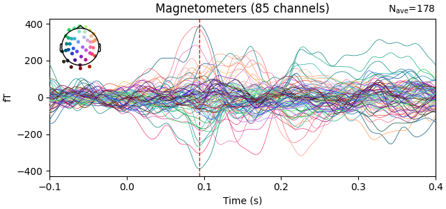
数据完成预处理后,现在可以在传感器层面观察到听觉诱发响应。
events = mne.find_events(raw, min_duration=0.1)
epochs = mne.Epochs(
    raw, events, tmin=-0.1, tmax=0.4, baseline=(-0.1, 0.0), verbose="error"
)
evoked = epochs.average()
t_peak = evoked.times[np.argmax(np.std(evoked.copy().pick("meg").data, axis=0))]
fig = evoked.plot_joint(picks="mag")
Finding events on: NI-TRIG
180 events found on stim channel NI-TRIG
Event IDs: [3]
Projections have already been applied. Setting proj attribute to True.
可视化配准#
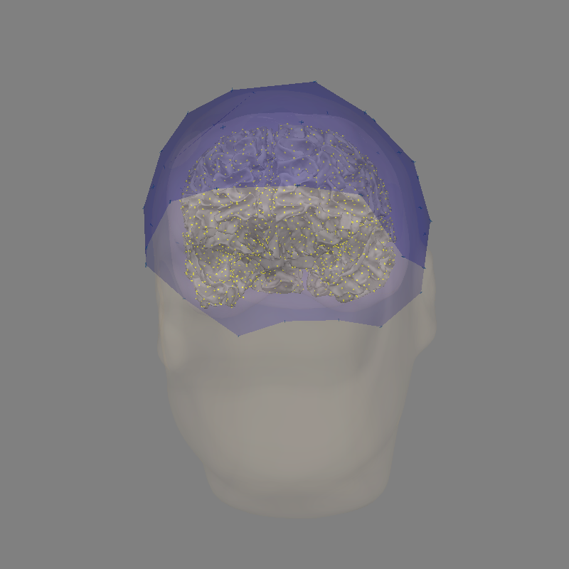
按设计,该数据集中的传感器已处于扫描仪 RAS 坐标系中。因此,我们可以通过计算 FreeSurfer MRI 坐标系与扫描仪 RAS 坐标系之间的变换,在 FreeSurfer MRI 坐标系中对其进行可视化:
mri = nib.load(subjects_dir / "sub-002" / "mri" / "T1.mgz")
trans = mri.header.get_vox2ras_tkr() @ np.linalg.inv(mri.affine)
trans[:3, 3] /= 1000.0  # nibabel uses mm, MNE uses m
trans = mne.transforms.Transform("head", "mri", trans)

bem = subjects_dir / subject / "bem" / f"{subject}-5120-bem-sol.fif"
src = subjects_dir / subject / "bem" / f"{subject}-oct-6-src.fif"
mne.viz.plot_alignment(
    evoked.info,
    subjects_dir=subjects_dir,
    subject=subject,
    trans=trans,
    surfaces={"head": 0.1, "inner_skull": 0.2, "white": 1.0},
    meg=["helmet", "sensors"],
    verbose="error",
    bem=bem,
    src=src,
)
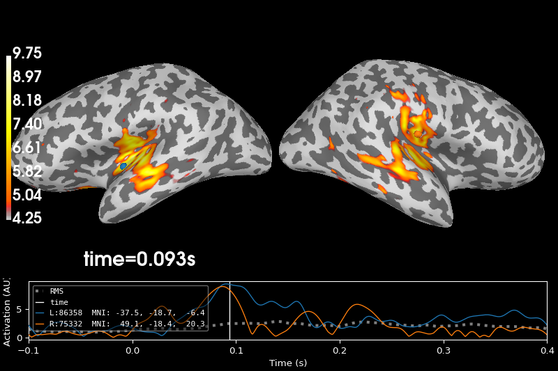
绘制逆解#
现在可以计算正向解和逆解:
fwd = mne.make_forward_solution(
    evoked.info,
    trans=trans,
    bem=bem,
    src=src,
    verbose=True,
)
noise_cov = mne.compute_covariance(epochs, tmax=0)
inv = mne.minimum_norm.make_inverse_operator(evoked.info, fwd, noise_cov, verbose=True)
stc = mne.minimum_norm.apply_inverse(
    evoked, inv, 1.0 / 9.0, method="dSPM", verbose=True
)
brain = stc.plot(
    hemi="split",
    size=(800, 400),
    initial_time=t_peak,
    subjects_dir=subjects_dir,
)
Source space          : /home/circleci/mne_data/auditory_OPM_stationary/derivatives/freesurfer/subjects/sub-002/bem/sub-002-oct-6-src.fif
MRI -> head transform : instance of Transform
Measurement data      : instance of Info
Conductor model   : /home/circleci/mne_data/auditory_OPM_stationary/derivatives/freesurfer/subjects/sub-002/bem/sub-002-5120-bem-sol.fif
Accurate field computations
Do computations in head coordinates
Free source orientations

Reading /home/circleci/mne_data/auditory_OPM_stationary/derivatives/freesurfer/subjects/sub-002/bem/sub-002-oct-6-src.fif...
Read 2 source spaces a total of 8196 active source locations

Coordinate transformation: MRI (surface RAS) -> head
    1.000000 0.000000 0.000000       0.50 mm
    0.000000 1.000000 0.000000      26.98 mm
    0.000000 0.000000 1.000000      -9.21 mm
    0.000000 0.000000 0.000000       1.00

Read 94 MEG channels from info
Read 8 MEG compensation channels from info
0 compensation data sets in info
Setting up compensation data...
    No compensation set. Nothing more to do.
105 coil definitions read
Coordinate transformation: MEG device -> head
    1.000000 0.000000 0.000000       0.00 mm
    0.000000 1.000000 0.000000       0.00 mm
    0.000000 0.000000 1.000000       0.00 mm
    0.000000 0.000000 0.000000       1.00
MEG coil definitions created in head coordinates.
Source spaces are now in head coordinates.

Setting up the BEM model using /home/circleci/mne_data/auditory_OPM_stationary/derivatives/freesurfer/subjects/sub-002/bem/sub-002-5120-bem-sol.fif...

Loading surfaces...

Loading the solution matrix...

Homogeneous model surface loaded.
Loaded linear collocation BEM solution from /home/circleci/mne_data/auditory_OPM_stationary/derivatives/freesurfer/subjects/sub-002/bem/sub-002-5120-bem-sol.fif
Employing the head->MRI coordinate transform with the BEM model.
BEM model sub-002-5120-bem-sol.fif is now set up


Source spaces are in head coordinates.
Checking that the sources are inside the surface (will take a few...)
Checking surface interior status for 4098 points...
    Found  535/4098 points inside  an interior sphere of radius   35.6 mm
    Found    0/4098 points outside an exterior sphere of radius   98.5 mm
    Found    0/3563 points outside using surface Qhull
    Found    0/3563 points outside using solid angles
    Total 4098/4098 points inside the surface
Interior check completed in 408.9 ms
Checking surface interior status for 4098 points...
    Found  501/4098 points inside  an interior sphere of radius   35.6 mm
    Found    0/4098 points outside an exterior sphere of radius   98.5 mm
    Found    0/3597 points outside using surface Qhull
    Found    0/3597 points outside using solid angles
    Total 4098/4098 points inside the surface
Interior check completed in 238.7 ms
Checking surface interior status for 94 points...
    Found  0/94 points inside  an interior sphere of radius   35.6 mm
    Found 30/94 points outside an exterior sphere of radius   98.5 mm
    Found 64/64 points outside using surface Qhull
    Found  0/ 0 points outside using solid angles
    Total 0/94 points inside the surface
Interior check completed in 0.8 ms

Composing the field computation matrix...
Computing MEG at 8196 source locations (free orientations)...

Finished.
Using data from preloaded Raw for 180 events and 3001 original time points ...
2 bad epochs dropped
    Created an SSP operator (subspace dimension = 8)
    Setting small MAG eigenvalues to zero (without PCA)
Reducing data rank from 85 -> 77
Estimating covariance using EMPIRICAL
Done.
Number of samples used : 106978
[done]
Converting forward solution to surface orientation
    Average patch normals will be employed in the rotation to the local surface coordinates....
    Converting to surface-based source orientations...
    [done]
info["bads"] and noise_cov["bads"] do not match, excluding bad channels from both
Computing inverse operator with 85 channels.
    85 out of 86 channels remain after picking
Selected 85 channels
Creating the depth weighting matrix...
    85 magnetometer or axial gradiometer channels
    limit = 7888/8196 = 10.028156
    scale = 1.9787e-10 exp = 0.8
Applying loose dipole orientations to surface source spaces: 0.2
Whitening the forward solution.
    Created an SSP operator (subspace dimension = 8)
Computing rank from covariance with rank=None
    Using tolerance 4.2e-14 (2.2e-16 eps * 85 dim * 2.2  max singular value)
    Estimated rank (mag): 77
    MAG: rank 77 computed from 85 data channels with 8 projectors
    Setting small MAG eigenvalues to zero (without PCA)
Creating the source covariance matrix
Adjusting source covariance matrix.
Computing SVD of whitened and weighted lead field matrix.
    largest singular value = 2.39473
    scaling factor to adjust the trace = 9.52253e+18 (nchan = 85 nzero = 8)
Preparing the inverse operator for use...
    Scaled noise and source covariance from nave = 1 to nave = 178
    Created the regularized inverter
    Created an SSP operator (subspace dimension = 8)
    Created the whitener using a noise covariance matrix with rank 77 (8 small eigenvalues omitted)
    Computing noise-normalization factors (dSPM)...
[done]
Applying inverse operator to "3"...
    Picked 85 channels from the data
    Computing inverse...
    Eigenleads need to be weighted ...
    Computing residual...
    Explained  90.3% variance
    Combining the current components...
    dSPM...
[done]
Using control points [4.25382465 4.85477031 9.75261481]
参考文献#
脚本总运行时间:(0 分钟 18.407 秒)