
非官方中文翻译
本页译自 MNE-Python 官方文档:
查看英文原文 ↗。
文档版权归 MNE Developers 所有(BSD-3-Clause)。
说明
转到末尾下载完整示例代码。
Brainstorm CTF 体模数据集教程#
这里我们针对 Brainstorm CTF 体模教程数据集,从原始数据计算诱发响应。作为对比,请参阅 [ 1 ] 以及:
参考文献#
# Authors: Eric Larson <larson.eric.d@gmail.com>
#
# License: BSD-3-Clause
# Copyright the MNE-Python contributors.
import warnings

import matplotlib.pyplot as plt
import numpy as np

import mne
from mne import fit_dipole
from mne.datasets.brainstorm import bst_phantom_ctf
from mne.io import read_raw_ctf

print(__doc__)
该数据由 CTF 系统以 2400 Hz 采集。
data_path = bst_phantom_ctf.data_path(verbose=True)

# Switch to these to use the higher-SNR data:
# raw_path = op.join(data_path, 'phantom_200uA_20150709_01.ds')
# dip_freq = 7.
raw_path = data_path / "phantom_20uA_20150603_03.ds"
dip_freq = 23.0
erm_path = data_path / "emptyroom_20150709_01.ds"
raw = read_raw_ctf(raw_path, preload=True)
ds directory : /home/circleci/mne_data/MNE-brainstorm-data/bst_phantom_ctf/phantom_20uA_20150603_03.ds
    res4 data read.
    hc data read.
    Separate EEG position data file read.
    Quaternion matching (desired vs. transformed):
      -0.39   74.35    0.00 mm <->   -0.39   74.35   -0.00 mm (orig :  -39.23   63.82 -204.07 mm) diff =    0.000 mm
       0.39  -74.35    0.00 mm <->    0.39  -74.35    0.00 mm (orig :   65.69  -41.53 -205.68 mm) diff =    0.000 mm
      75.00    0.00    0.00 mm <->   75.00   -0.00    0.00 mm (orig :   64.32   61.80 -226.08 mm) diff =    0.000 mm
    Coordinate transformations established.
    Polhemus data for 3 HPI coils added
    Device coordinate locations for 3 HPI coils added
    Measurement info composed.
Finding samples for /home/circleci/mne_data/MNE-brainstorm-data/bst_phantom_ctf/phantom_20uA_20150603_03.ds/phantom_20uA_20150603_03.meg4:
    System clock channel is available, checking which samples are valid.
    10 x 2400 = 24000 samples from 304 chs
Current compensation grade : 3
Reading 0 ... 23999  =      0.000 ...    10.000 secs...
正弦信号由通道 HDAC006 产生,因此我们可以利用该通道获得精确的时间信息。
sinusoid, times = raw[raw.ch_names.index("HDAC006-4408")]
plt.figure()
plt.plot(times[times < 1.0], sinusoid.T[times < 1.0])
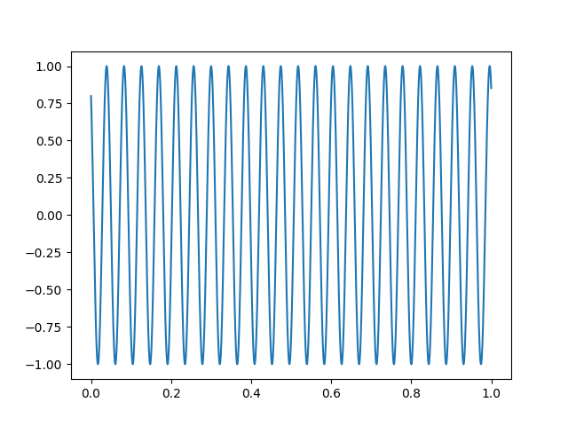
我们对该正弦信号做阈值处理,从而创建一些事件。
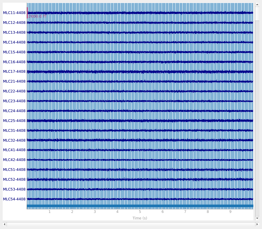
CTF 软件补偿的效果相当不错:
raw.plot()
Using qt as 2D backend.
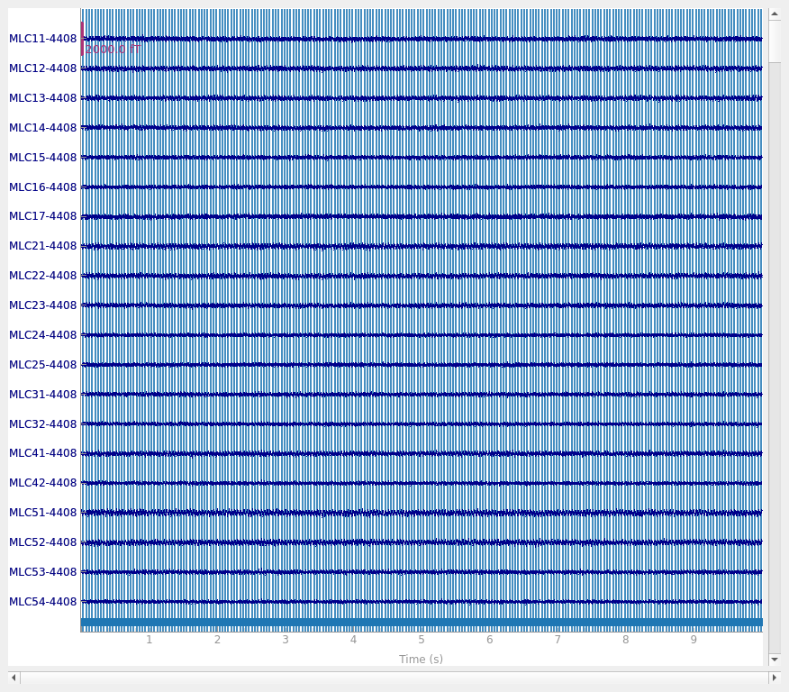
但在这里,使用时空(tSSS)Maxwell 滤波可以获得稍好的噪声抑制、更低的定位偏差以及更高的偶极子拟合优度:
raw.apply_gradient_compensation(0)  # must un-do software compensation first
mf_kwargs = dict(origin=(0.0, 0.0, 0.0), st_duration=10.0, st_overlap=True)
raw = mne.preprocessing.maxwell_filter(raw, **mf_kwargs)
raw.plot()
Compensator constructed to change 3 -> 0
Applying compensator to loaded data
Maxwell filtering raw data
    No bad MEG channels
    Processing 0 gradiometers and 299 magnetometers (of which 290 are actually KIT gradiometers)
    Using origin 0.0, 0.0, 0.0 mm in the head frame
    Processing data using tSSS with st_duration=10.0
    Using loaded raw data
        Using 86/95 harmonic components for    0.000  (71/80 in, 15/15 out)
    Processing    1 data chunk of (at least) 10.0 s with 5.0 s overlap and hann windowing
        Using 86/95 harmonic components for    0.000  (71/80 in, 15/15 out)
        Projecting  8 intersecting tSSS components for    0.000 -   10.000 s
        Using 86/95 harmonic components for    0.000  (71/80 in, 15/15 out)
[done]
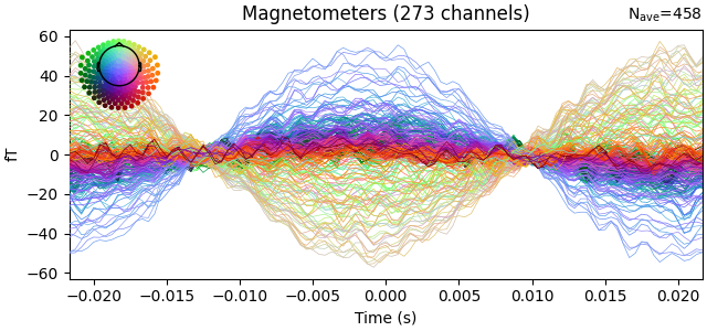
我们选择的 tmin 和 tmax 应恰好覆盖一个周期,因此在创建诱发数据时,我们可以采用一种不太常见的做法:用整个 epoch 做基线校正。随后我们还将数据裁剪到单个时间点(@t=0),因为这一点正是信号的峰值。
tmin = -0.5 / dip_freq
tmax = -tmin
epochs = mne.Epochs(
    raw, events, event_id=1, tmin=tmin, tmax=tmax, baseline=(None, None)
)
evoked = epochs.average()
evoked.plot(time_unit="s")
evoked.crop(0.0, 0.0)
Not setting metadata
460 matching events found
Setting baseline interval to [-0.021666666666666667, 0.021666666666666667] s
Applying baseline correction (mode: mean)
0 projection items activated
Removing 5 compensators from info because not all compensation channels were picked.
Removing 5 compensators from info because not all compensation channels were picked.
Removing 5 compensators from info because not all compensation channels were picked.
我们使用球形头几何模型,并查看坐标对齐情况和球体位置。
sphere = mne.make_sphere_model(r0=(0.0, 0.0, 0.0), head_radius=0.08)

mne.viz.plot_alignment(
    raw.info, subject="sample", meg="helmet", bem=sphere, dig=True, surfaces=["brain"]
)
del raw, epochs
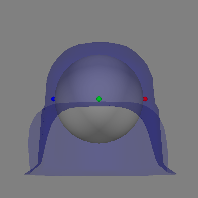
Equiv. model fitting -> RV = 0.00347813 %%
mu1 = 0.944815    lambda1 = 0.13694
mu2 = 0.667658    lambda2 = 0.683728
mu3 = -0.286487    lambda3 = -0.0102992
Set up EEG sphere model with scalp radius    80.0 mm

Getting helmet for system CTF_275
为了进行偶极子拟合,我们使用由空房间记录提供的协方差。
raw_erm = read_raw_ctf(erm_path).apply_gradient_compensation(0)
raw_erm = mne.preprocessing.maxwell_filter(raw_erm, coord_frame="meg", **mf_kwargs)
cov = mne.compute_raw_covariance(raw_erm)
del raw_erm

with warnings.catch_warnings(record=True):
    # ignore warning about data rank exceeding that of info (75 > 71)
    warnings.simplefilter("ignore")
    dip, residual = fit_dipole(evoked, cov, sphere, verbose=True)
ds directory : /home/circleci/mne_data/MNE-brainstorm-data/bst_phantom_ctf/emptyroom_20150709_01.ds
    res4 data read.
    hc data read.
    Separate EEG position data file read.
    Quaternion matching (desired vs. transformed):
      -0.00   74.50    0.00 mm <->   -0.00   74.50   -0.00 mm (orig :  -50.17   57.61 -188.51 mm) diff =    0.000 mm
       0.00  -74.50    0.00 mm <->    0.00  -74.50    0.00 mm (orig :   60.49  -42.15 -190.81 mm) diff =    0.000 mm
      74.66    0.00    0.00 mm <->   74.66   -0.00    0.00 mm (orig :   53.03   61.29 -209.99 mm) diff =    0.000 mm
    Coordinate transformations established.
    Polhemus data for 3 HPI coils added
    Device coordinate locations for 3 HPI coils added
    Measurement info composed.
Finding samples for /home/circleci/mne_data/MNE-brainstorm-data/bst_phantom_ctf/emptyroom_20150709_01.ds/emptyroom_20150709_01.meg4:
    System clock channel is available, checking which samples are valid.
    100 x 600 = 60000 samples from 304 chs
Current compensation grade : 3
Compensator constructed to change 3 -> 0
Maxwell filtering raw data
    No bad MEG channels
    Processing 0 gradiometers and 299 magnetometers (of which 290 are actually KIT gradiometers)
    Using origin 0.0, 0.0, 0.0 mm in the meg frame (1.3, -8.8, -2.8 mm in the head frame)
    Processing data using tSSS with st_duration=10.0
    Loading raw data from disk
        Using 90/95 harmonic components for    0.000  (75/80 in, 15/15 out)
    Processing   19 data chunks of (at least) 10.0 s with 5.0 s overlap and hann windowing
        Using 90/95 harmonic components for    0.000  (75/80 in, 15/15 out)
        Projecting  8 intersecting tSSS components for    0.000 -    9.998 s
        Projecting  8 intersecting tSSS components for    5.000 -   14.998 s
        Projecting  8 intersecting tSSS components for   10.000 -   19.998 s
        Projecting  8 intersecting tSSS components for   15.000 -   24.998 s
        Projecting  8 intersecting tSSS components for   20.000 -   29.998 s
        Projecting  8 intersecting tSSS components for   25.000 -   34.998 s
        Projecting  8 intersecting tSSS components for   30.000 -   39.998 s
        Projecting  8 intersecting tSSS components for   35.000 -   44.998 s
        Projecting  9 intersecting tSSS components for   40.000 -   49.998 s
        Projecting  9 intersecting tSSS components for   45.000 -   54.998 s
        Projecting  8 intersecting tSSS components for   50.000 -   59.998 s
        Projecting  8 intersecting tSSS components for   55.000 -   64.998 s
        Projecting  7 intersecting tSSS components for   60.000 -   69.998 s
        Projecting  8 intersecting tSSS components for   65.000 -   74.998 s
        Projecting  9 intersecting tSSS components for   70.000 -   79.998 s
        Projecting  8 intersecting tSSS components for   75.000 -   84.998 s
        Projecting  9 intersecting tSSS components for   80.000 -   89.998 s
        Projecting  9 intersecting tSSS components for   85.000 -   94.998 s
        Projecting  8 intersecting tSSS components for   90.000 -   99.998 s
        Using 90/95 harmonic components for    0.000  (75/80 in, 15/15 out)
[done]
Using up to 500 segments
Number of samples used : 60000
[done]
BEM               : <ConductorModel | Sphere (3 layers): r0=[0.0, 0.0, 0.0] R=80 mm>
MRI transform     : identity
Sphere model      : origin at (   0.00    0.00    0.00) mm, rad =    0.1 mm
Guess grid        :   20.0 mm
Guess mindist     :    5.0 mm
Guess exclude     :   20.0 mm
Using normal MEG coil definitions.
Noise covariance  : <Covariance | kind : full, shape : (273, 273), range : [-4.1e-28, +1.2e-27], n_samples : 59999>

Coordinate transformation: MRI (surface RAS) -> head
    1.000000 0.000000 0.000000       0.00 mm
    0.000000 1.000000 0.000000       0.00 mm
    0.000000 0.000000 1.000000       0.00 mm
    0.000000 0.000000 0.000000       1.00
Coordinate transformation: MEG device -> head
    0.999939 -0.002039 -0.010868      -2.00 mm
    -0.001115 0.959234 -0.282612     -20.74 mm
    0.011001 0.282607 0.959173       9.38 mm
    0.000000 0.000000 0.000000       1.00
0 bad channels total
Read 299 MEG channels from info
Read 26 MEG compensation channels from info
5 compensation data sets in info
Setting up compensation data...
    No compensation set. Nothing more to do.
105 coil definitions read
Coordinate transformation: MEG device -> head
    0.999939 -0.002039 -0.010868      -2.00 mm
    -0.001115 0.959234 -0.282612     -20.74 mm
    0.011001 0.282607 0.959173       9.38 mm
    0.000000 0.000000 0.000000       1.00
MEG coil definitions created in head coordinates.
Decomposing the sensor noise covariance matrix...
Removing 5 compensators from info because not all compensation channels were picked.
Computing rank from covariance with rank=None
    Using tolerance 1.9e-15 (2.2e-16 eps * 273 dim * 0.031  max singular value)
    Estimated rank (mag): 75
    MAG: rank 75 computed from 273 data channels with 0 projectors
    Setting small MAG eigenvalues to zero (without PCA)
    Created the whitener using a noise covariance matrix with rank 75 (198 small eigenvalues omitted)

---- Computing the forward solution for the guesses...
Making a spherical guess space with radius    72.0 mm...
Filtering (grid =     20 mm)...
Surface CM = (   0.0    0.0    0.0) mm
Surface fits inside a sphere with radius   72.0 mm
Surface extent:
    x =  -72.0 ...   72.0 mm
    y =  -72.0 ...   72.0 mm
    z =  -72.0 ...   72.0 mm
Grid extent:
    x =  -80.0 ...   80.0 mm
    y =  -80.0 ...   80.0 mm
    z =  -80.0 ...   80.0 mm
729 sources before omitting any.
178 sources after omitting infeasible sources not within 20.0 - 72.0 mm.
Source spaces are in MRI coordinates.
Checking that the sources are inside the surface and at least    5.0 mm away (will take a few...)
    8 source space point omitted because of the    5.0-mm distance limit.
170 sources remaining after excluding the sources outside the surface and less than    5.0 mm inside.
Go through all guess source locations...
[done 170 sources]
---- Fitted :     0.0 ms
No projector specified for this dataset. Please consider the method self.add_proj.
1 time points fitted
将实际位置与估计位置进行比较。
expected_pos = np.array([18.0, 0.0, 49.0])
diff = np.sqrt(np.sum((dip.pos[0] * 1000 - expected_pos) ** 2))
print(f"Actual pos:     {np.array_str(expected_pos, precision=1)} mm")
print(f"Estimated pos:  {np.array_str(dip.pos[0] * 1000, precision=1)} mm")
print(f"Difference:     {diff:0.1f} mm")
print(f"Amplitude:      {1e9 * dip.amplitude[0]:0.1f} nAm")
print(f"GOF:            {dip.gof[0]:0.1f} %")
Actual pos:     [18.  0. 49.] mm
Estimated pos:  [18.5 -2.2 44.6] mm
Difference:     5.0 mm
Amplitude:      10.1 nAm
GOF:            96.4 %
脚本总运行时间:(0 分 11.445 秒)