在剔除前探索分段质量#

本示例展示识别可能含伪迹的分段并剔除坏分段的方法：使用峰峰值幅度、方差与峰度计算每个分段的离群分数——受 FASTER [1] 与 Delorme 等 [2] 启发——并据此把分段从最干净到最嘈杂排序，为剔除决策提供依据。

# Authors: Aman Srivastava
#
# License: BSD-3-Clause
# Copyright the MNE-Python contributors.

import matplotlib.pyplot as plt
import numpy as np
from scipy.stats import kurtosis

import mne
from mne.datasets import eegbci

print(__doc__)

加载 EEGBCI 数据集并创建分段#

raw_fname = eegbci.load_data(subjects=3, runs=(3,))[0]
raw = mne.io.read_raw(raw_fname, preload=True)
eegbci.standardize(raw)
montage = mne.channels.make_standard_montage("spherical_1005")
raw.set_montage(montage)

events, event_id = mne.events_from_annotations(raw)
epochs = mne.Epochs(raw, events, tmin=-0.2, tmax=0.5, preload=True, baseline=(None, 0))

Extracting EDF parameters from /home/circleci/mne_data/MNE-eegbci-data/files/eegmmidb/1.0.0/S003/S003R03.edf...
Setting channel info structure...
Creating raw.info structure...
Reading 0 ... 19999  =      0.000 ...   124.994 secs...
Used Annotations descriptions: ['T0', 'T1', 'T2']
Not setting metadata
30 matching events found
Setting baseline interval to [-0.2, 0.0] s
Applying baseline correction (mode: mean)
0 projection items activated
Using data from preloaded Raw for 30 events and 113 original time points ...
1 bad epochs dropped

计算每个分段的离群分数#

峰峰值幅度、方差与峰度按分段计算。每个特征用跨分段的绝对中位差做稳健 z 分数化，再平均为归一化到 [0, 1] 的单一离群分数。分数接近 1 表示该分段很可能含伪迹。

data = epochs.get_data()  # (n_epochs, n_channels, n_times)

ptp = np.ptp(data, axis=-1).mean(axis=-1)
var = data.var(axis=-1).mean(axis=-1)
kurt = np.array([kurtosis(data[i].ravel()) for i in range(len(data))])

features = np.column_stack([ptp, var, kurt])
median = np.median(features, axis=0)
mad = np.median(np.abs(features - median), axis=0) + 1e-10
z = np.abs((features - median) / mad)

raw_score = z.mean(axis=-1)
scores = (raw_score - raw_score.min()) / (raw_score.max() - raw_score.min() + 1e-10)

判定离群分段#

下面把分段从最干净到最嘈杂排序。需要找到合适阈值来标记可能含伪迹的分段，所用阈值会随数据集与分析目标而变。图中展示两个示例阈值：较宽松的 0.6 与较严格的 0.3。

fig, ax = plt.subplots(layout="constrained")
sorted_idx = np.argsort(scores)
ax.bar(np.arange(len(scores)), scores[sorted_idx], color="steelblue")
ax.axhline(0.6, color="red", linestyle="--", label="More lenient threshold (0.6)")
ax.axhline(0.3, color="orange", linestyle="--", label="Stricter threshold (0.3)")
ax.set(
    xlabel="Epoch (sorted by score)",
    ylabel="Outlier score",
    title="Epoch quality scores (0 = clean, 1 = likely artifact)",
)
ax.legend()

for threshold in [0.6, 0.3]:
    bad_epochs = np.where(scores > threshold)[0]
    print(
        f"Threshold {threshold}: {len(bad_epochs)} epochs flagged "
        f"out of {len(epochs)} total"
    )

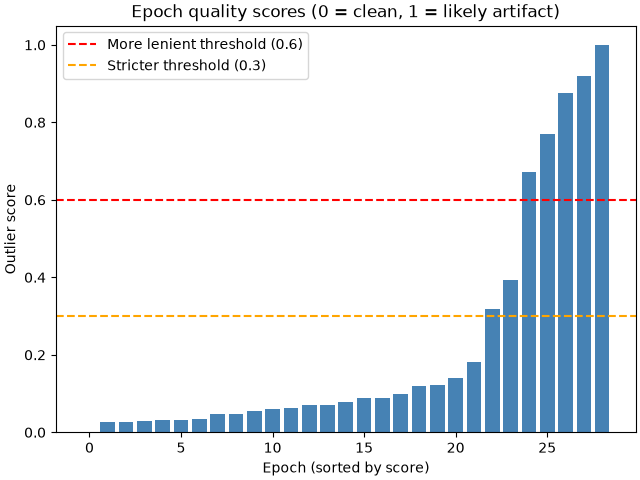
Epoch quality scores (0 = clean, 1 = likely artifact)

Threshold 0.6: 5 epochs flagged out of 29 total
Threshold 0.3: 7 epochs flagged out of 29 total

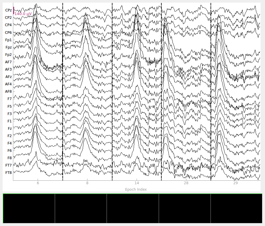
可用 mne.Epochs.plot() 方法检查被阈值标记的分段，这是确定最佳阈值的关键步骤。先看分数最差（≥ 0.6）的分段，其中包含若干幅度尖峰。

picks = np.arange(17, 40, dtype=int)  # channels with notable amplitude spikes
epochs[np.where(scores >= 0.6)[0]].plot(
    picks=picks, title="Scores ≥ 0.6", scalings=dict(eeg=70e-6), n_channels=len(picks)
)

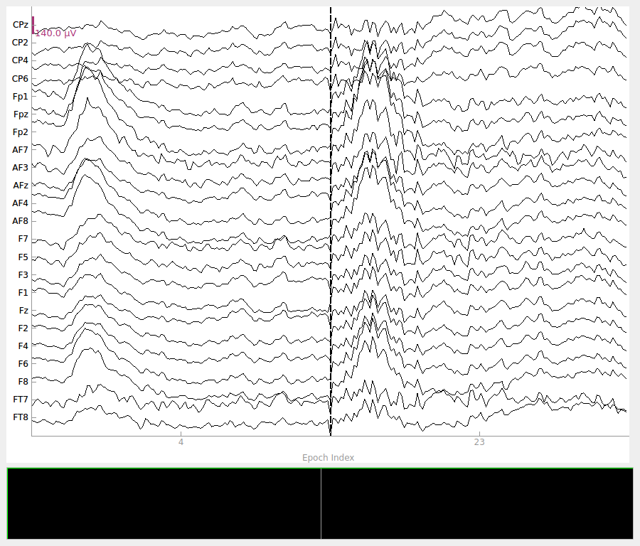
相比之下，阈值 0.3 会捕获伪迹活动较轻的分段，把它们排除在分析之外可能过于保守。

epochs[np.where((scores >= 0.3) & (scores < 0.6))[0]].plot(
    picks=picks,
    title="0.3 ≤ scores < 0.6",
    scalings=dict(eeg=70e-6),
    n_channels=len(picks),
)

剔除可疑分段#

目视检查后，可用 mne.Epochs.drop() 方法丢弃坏分段。这里移除分数最差（≥ 0.6）、含强烈伪迹活动的分段，剩余的良好分段可用于后续分析。

修复并保留含伪迹的分段

本例中大的额叶偏转很可能是眨眼伪迹，因此丢弃并非唯一选择。对这类伪迹，通常更可取的是修复数据并保留更多分段，例如使用基于 ICA 或回归的伪迹校正。

epochs.drop(np.where(scores >= 0.6)[0])
print(f"Epochs remaining after dropping scores ≥ 0.6: {len(epochs)}")

Dropped 5 epochs: 5, 7, 13, 27, 28
Epochs remaining after dropping scores ≥ 0.6: 24

参考文献#

图库由 Sphinx-Gallery 生成