
说明
转到末尾下载完整示例代码。
将 Epochs 导出为 Pandas DataFrame#
本教程展示如何将 Epochs 对象中的数据导出为 Pandas DataFrame,并应用典型的 Pandas split-apply-combine(拆分-应用-合并)工作流,考察各个 epoch 与各种条件下反应最大值的潜伏期。
我们将使用 Sample 数据集,但加载的是原始文件的一个版本,该版本已经过滤波和降采样,并且其 EEG 通道已施加平均参考。和往常一样,我们先导入所需的模块并加载数据:
# Authors: The MNE-Python contributors.
# License: BSD-3-Clause
# Copyright the MNE-Python contributors.
import matplotlib.pyplot as plt
import seaborn as sns

import mne

sample_data_folder = mne.datasets.sample.data_path()
sample_data_raw_file = (
    sample_data_folder / "MEG" / "sample" / "sample_audvis_filt-0-40_raw.fif"
)
raw = mne.io.read_raw_fif(sample_data_raw_file, verbose=False)
接下来,我们从文件中加载事件列表,用事件字典将其映射为条件名称,设置一些信号拒绝阈值(参见 Rejecting Epochs based on peak-to-peak channel amplitude),然后将连续数据分割为 epoch:
sample_data_events_file = (
    sample_data_folder / "MEG" / "sample" / "sample_audvis_filt-0-40_raw-eve.fif"
)
events = mne.read_events(sample_data_events_file)

event_dict = {
    "auditory/left": 1,
    "auditory/right": 2,
    "visual/left": 3,
    "visual/right": 4,
}

reject_criteria = dict(
    mag=3000e-15,  # 3000 fT
    grad=3000e-13,  # 3000 fT/cm
    eeg=100e-6,  # 100 µV
    eog=200e-6,
)  # 200 µV

tmin, tmax = (-0.2, 0.5)  # epoch from 200 ms before event to 500 ms after it
baseline = (None, 0)  # baseline period from start of epoch to time=0

epochs = mne.Epochs(
    raw,
    events,
    event_dict,
    tmin,
    tmax,
    proj=True,
    baseline=baseline,
    reject=reject_criteria,
    preload=True,
)
del raw
Not setting metadata
288 matching events found
Setting baseline interval to [-0.19979521315838786, 0.0] s
Applying baseline correction (mode: mean)
Created an SSP operator (subspace dimension = 4)
4 projection items activated
Loading data for 288 events and 106 original time points ...
    Rejecting  epoch based on EEG : ['EEG 003']
    Rejecting  epoch based on EEG : ['EEG 001', 'EEG 002', 'EEG 003', 'EEG 004', 'EEG 006', 'EEG 007']
    Rejecting  epoch based on EEG : ['EEG 001', 'EEG 002', 'EEG 003', 'EEG 007']
    Rejecting  epoch based on EEG : ['EEG 001']
    Rejecting  epoch based on EEG : ['EEG 003', 'EEG 007']
    Rejecting  epoch based on EEG : ['EEG 007']
    Rejecting  epoch based on EEG : ['EEG 003', 'EEG 007']
    Rejecting  epoch based on EEG : ['EEG 007']
    Rejecting  epoch based on MAG : ['MEG 1411', 'MEG 1421', 'MEG 1441']
    Rejecting  epoch based on MAG : ['MEG 1711']
    Rejecting  epoch based on EEG : ['EEG 001', 'EEG 002', 'EEG 003', 'EEG 007']
    Rejecting  epoch based on EEG : ['EEG 007']
    Rejecting  epoch based on MAG : ['MEG 1411', 'MEG 1421']
    Rejecting  epoch based on MAG : ['MEG 1711']
    Rejecting  epoch based on EOG : ['EOG 061']
    Rejecting  epoch based on EEG : ['EEG 008']
    Rejecting  epoch based on EEG : ['EEG 008']
    Rejecting  epoch based on EOG : ['EOG 061']
    Rejecting  epoch based on EEG : ['EEG 007', 'EEG 008']
    Rejecting  epoch based on EEG : ['EEG 001', 'EEG 002', 'EEG 003', 'EEG 007']
    Rejecting  epoch based on EEG : ['EEG 001', 'EEG 003', 'EEG 007']
    Rejecting  epoch based on MAG : ['MEG 1411', 'MEG 1421']
    Rejecting  epoch based on MAG : ['MEG 1411']
    Rejecting  epoch based on EEG : ['EEG 001', 'EEG 002', 'EEG 003', 'EEG 007']
    Rejecting  epoch based on EEG : ['EEG 001', 'EEG 002', 'EEG 003', 'EEG 007']
    Rejecting  epoch based on EEG : ['EEG 007']
    Rejecting  epoch based on EEG : ['EEG 003', 'EEG 007']
    Rejecting  epoch based on EEG : ['EEG 003', 'EEG 007']
    Rejecting  epoch based on EEG : ['EEG 007']
    Rejecting  epoch based on MAG : ['MEG 1331', 'MEG 1421']
    Rejecting  epoch based on EEG : ['EEG 007']
    Rejecting  epoch based on EOG : ['EOG 061']
    Rejecting  epoch based on EEG : ['EEG 001', 'EEG 002', 'EEG 003', 'EEG 007']
    Rejecting  epoch based on EEG : ['EEG 001', 'EEG 002', 'EEG 003', 'EEG 007']
    Rejecting  epoch based on EEG : ['EEG 001', 'EEG 002', 'EEG 003', 'EEG 007']
35 bad epochs dropped
将 Epochs 对象转换为 DataFrame#
有了 Epochs 对象之后,将其转换为 DataFrame 就很简单:只需调用 epochs.to_data_frame()。每个通道的数据都会成为新 DataFrame 的一列,此外还有三列分别记录事件名称、epoch 编号和采样时间。这里我们只展示前几行和前几列:
df = epochs.to_data_frame()
df.iloc[:5, :10]
缩放时间与通道数值#
默认情况下,时间值会从秒转换为毫秒,然后四舍五入到最接近的整数;如果你不希望这样,可以传入 time_format=None,以秒为单位将时间保留为 float 浮点值,也可以通过 time_format='timedelta' 将其转换为 Timedelta 值。
另请注意,默认情况下通道测量值会被缩放,使 EEG 数据转换为 µV、磁力计数据转换为 fT、梯度计数据转换为 fT/cm。这些缩放可以通过 scalings 参数自定义,或者通过传入 scalings=dict(eeg=1, mag=1, grad=1) 来取消。
df = epochs.to_data_frame(time_format=None, scalings=dict(eeg=1, mag=1, grad=1))
df.iloc[:5, :10]
注意,时间值不再是整数,而且与前一个 DataFrame 相比,通道数值变化了好几个数量级。
设置索引#
还可以通过向 index 参数传入一个字符串或字符串列表,将一个或多个指示列(事件名称、epoch 编号和采样时间)移入索引。这里我们还会演示 time_format='timedelta' 的效果,在“time”列中生成 Timedelta 值。
df = epochs.to_data_frame(index=["condition", "epoch"], time_format="timedelta")
df.iloc[:5, :10]
宽格式与长格式 DataFrame#
另一个参数 long_format 决定每个通道的数据是放在 DataFrame 的单独一列中(long_format=False),还是将测量值透视为单个 'value' 列,并额外增加一列用于指示通道名称(long_format=True)。传入 long_format=True 还会额外创建一列 ch_type,用于指示通道类型。
long_df = epochs.to_data_frame(time_format=None, index="condition", long_format=True)
long_df.head()
Converting "epoch" to "category"...
Converting "channel" to "category"...
Converting "ch_type" to "category"...
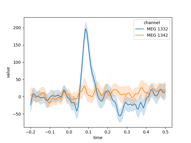
在使用其他 Python 模块进行后续分析或绘图时,以长格式生成 DataFrame 会很有帮助。例如,这里我们取出“auditory/left”条件的数据,挑选几个 MEG 通道,并使用 seaborn.lineplot() 自动绘制每个通道的均值和置信带,其中的置信度是在所选条件的各个 epoch 上计算得到的:
plt.figure()
channels = ["MEG 1332", "MEG 1342"]
data = long_df.loc["auditory/left"].query("channel in @channels")
# convert channel column (CategoryDtype → string; for a nicer-looking legend)
data["channel"] = data["channel"].astype(str)
data.reset_index(drop=True, inplace=True)  # speeds things up
sns.lineplot(x="time", y="value", hue="channel", data=data)
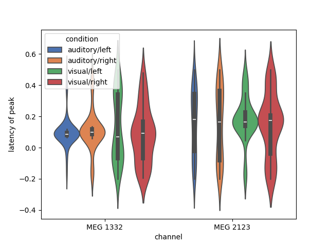
现在,我们还可以充分利用 Pandas 的强大功能来对数据分组和变换。这里,我们找出 2 个梯度计(一个靠近听觉皮层,一个靠近视觉皮层)峰值激活的潜伏期,并用 violinplot() 绘制每个通道峰值出现时间的分布:
plt.figure()
df = epochs.to_data_frame(time_format=None)
peak_latency = (
    df.filter(regex=r"condition|epoch|MEG 1332|MEG 2123")
    .groupby(["condition", "epoch"])
    .aggregate(lambda x: df["time"].iloc[x.idxmax()])
    .reset_index()
    .melt(
        id_vars=["condition", "epoch"], var_name="channel", value_name="latency of peak"
    )
)
ax = sns.violinplot(
    x="channel",
    y="latency of peak",
    hue="condition",
    data=peak_latency,
    palette="deep",
    saturation=1,
)
脚本总运行时间:(0 分钟 4.167 秒)