非官方中文翻译本页译自 MNE-Python 官方文档：查看英文原文 ↗。文档版权归 MNE Developers 所有（BSD-3-Clause）。

注意

转到末尾下载完整示例代码。

使用回归修复伪迹#

本教程介绍如何使用回归方法去除伪迹，方法原理参见 Gratton et al. (1983) [ 1 ] 和 Croft & Barry (2000) [ 2 ] 。

一般来说，只要某种伪迹在传感器上产生的时间波形能够被某个参考信号准确反映，就可以通过回归将其去除。双极 EOG 通道记录到的眨眼伪迹就是一个很好的例子，因此我们在本教程中以此进行演示。

尽管双极 ECG 电极能够很好地记录心电信号，但基于回归去除 ECG 伪迹通常效果不佳。这可能是因为心脏就像一个旋转的偶极子，因此从 ECG 电极位置记录到的 ECG 通道时间波形，并不能反映在每个 MEG 通道上表现出的相同时间动态（MEG 通道测量的是相关磁场矢量场的某个分量）。对于 ECG，使用 ICA 或 SSP 等其他方法可能效果更好。

此外，回归方法通常用于通道数量较少、且不适合去除整个信号成分的场合。因此，大多数相关文献针对的都是 EEG，该技术很少应用于 MEG。基于这一原因，我们在本教程中只对 EEG 数据进行分析。

准备数据#

和以往一样，我们首先导入必要的 Python 模块并加载数据。MNE-Sample 数据集中有一些明显而粗大的眨眼伪迹，尤其是在呈现视觉刺激期间。

# Authors: The MNE-Python contributors.
# License: BSD-3-Clause
# Copyright the MNE-Python contributors.

import numpy as np

import mne
from mne.preprocessing import EOGRegression

data_path = mne.datasets.sample.data_path()
raw_fname = data_path / "MEG" / "sample" / "sample_audvis_raw.fif"
raw = mne.io.read_raw_fif(raw_fname)
raw.pick(["eeg", "eog", "stim"])
raw.load_data()

# The regression technique works regardless of chosen reference. However, it is
# important to choose a reference before proceeding with the analysis.
raw.set_eeg_reference("average")

# Removing slow drifts makes for more stable regression coefficients. Make sure
# to apply the same filter to both EEG and EOG channels!
raw.filter(0.3, 40)

# make epochs
events = mne.find_events(raw)
event_id = {"visual/left": 3, "visual/right": 4}
epochs = mne.Epochs(raw, events, event_id=event_id, preload=True)

Opening raw data file /home/circleci/mne_data/MNE-sample-data/MEG/sample/sample_audvis_raw.fif...
    Read a total of 3 projection items:
        PCA-v1 (1 x 102)  idle
        PCA-v2 (1 x 102)  idle
        PCA-v3 (1 x 102)  idle
    Range : 25800 ... 192599 =     42.956 ...   320.670 secs
Ready.
Reading 0 ... 166799  =      0.000 ...   277.714 secs...
EEG channel type selected for re-referencing
Applying average reference.
Applying a custom ('EEG',) reference.
Filtering raw data in 1 contiguous segment
Setting up band-pass filter from 0.3 - 40 Hz

FIR filter parameters
---------------------
Designing a one-pass, zero-phase, non-causal bandpass filter:
- Windowed time-domain design (firwin) method
- Hamming window with 0.0194 passband ripple and 53 dB stopband attenuation
- Lower passband edge: 0.30
- Lower transition bandwidth: 0.30 Hz (-6 dB cutoff frequency: 0.15 Hz)
- Upper passband edge: 40.00 Hz
- Upper transition bandwidth: 10.00 Hz (-6 dB cutoff frequency: 45.00 Hz)
- Filter length: 6607 samples (11.000 s)

Finding events on: STI 014
320 events found on stim channel STI 014
Event IDs: [ 1  2  3  4  5 32]
Not setting metadata
144 matching events found
Setting baseline interval to [-0.19979521315838786, 0.0] s
Applying baseline correction (mode: mean)
0 projection items activated
Using data from preloaded Raw for 144 events and 421 original time points ...
0 bad epochs dropped

可视化原始数据#

我们首先查看未施加任何校正的 Evoked 数据（对所有 epochs 取平均的结果）。

# we'll try to keep a consistent ylim across figures
plot_kwargs = dict(picks="all", ylim=dict(eeg=(-10, 10), eog=(-5, 15)))

# plot the evoked for the EEG and the EOG sensors
fig = epochs.average("all").plot(**plot_kwargs)
fig.set_size_inches(6, 6)

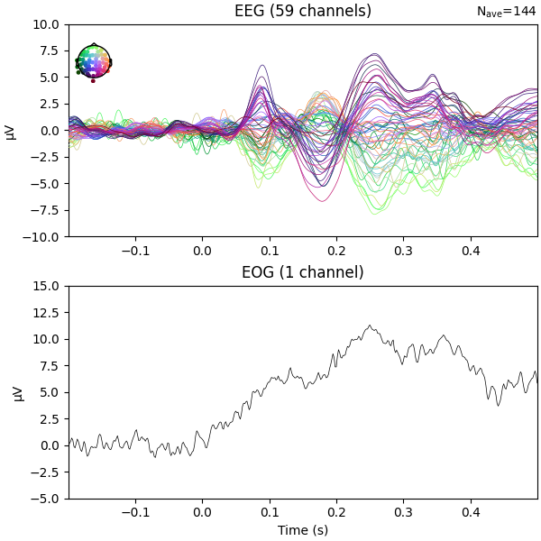
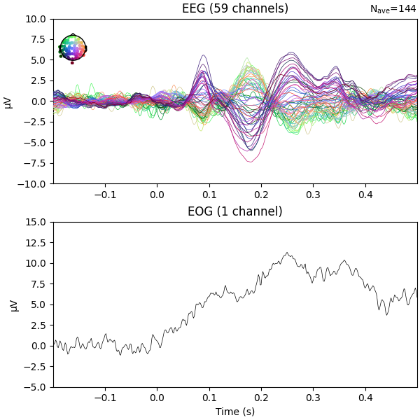
可以看到存在一些 EOG 活动，很可能已混入 EEG 诱发响应中。在大约 250 毫秒处这一点尤为明显。下面我们应用回归，从 EEG 信号中减去 EOG 信号，以对其进行清理。

计算并应用 EOG 回归#

现在，我们来比较回归去除 EOG 信号前后的诱发响应。首先尝试普通回归，然后再探索更高级的技术。

# Perform regression using the EOG sensor as independent variable and the EEG
# sensors as dependent variables.
model_plain = EOGRegression(picks="eeg", picks_artifact="eog").fit(epochs)
fig = model_plain.plot(vlim=(None, 0.4))  # regression coefficients as topomap
fig.set_size_inches(3, 2)

No projector specified for this dataset. Please consider the method self.add_proj.

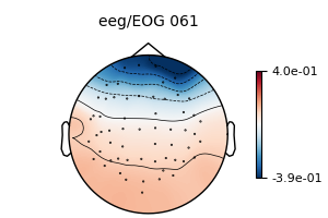
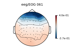
回归系数反映了每个 EEG 传感器与 EOG 传感器之间的线性关系。请注意，枕区传感器呈正相关，这是因为在上面加载数据时我们设置了平均参考（common-average reference）。

现在，我们可以使用这些系数从 EEG 信号中减去 EOG 信号了。

epochs_clean_plain = model_plain.apply(epochs)
# After regression, we should redo the baseline correction
epochs_clean_plain.apply_baseline()
# Show the evoked potential computed on the corrected data
fig = epochs_clean_plain.average("all").plot(**plot_kwargs)
fig.set_size_inches(6, 6)

No projector specified for this dataset. Please consider the method self.add_proj.
Applying baseline correction (mode: mean)

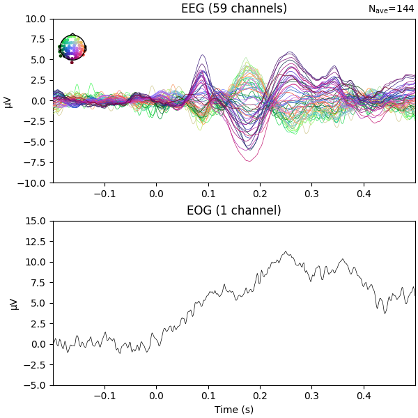
从 EEG 信号中回归去除 EOG 信号后，大约 250 毫秒处部分由眼动伪迹引起的峰值减小了。

在 MNE-Sample 数据集中，没有特别不稳定的数据片段，因此基本回归形式就能得到稳健的系数。但并非每个数据集都是如此，下面我们探索一些可能改善回归系数估计的变体方法。

一个潜在问题是，EOG 传感器不仅会采集到眼动伪迹，还会采集到少量 EEG 信号。这意味着，如果 EOG 传感器放置得离 EEG 传感器太近，我们容易高估回归系数。不过，我们可以应用一种校正来缓解这一问题。

回归前先从 epoch 数据中减去诱发响应#

Gratton et al. (1983) [ 1 ] 建议在减去诱发响应后的 epoch 数据上计算回归系数。其思路是：与研究相关的 EEG 信号成分都包含在诱发响应中，去除这些成分后，剩下的基本都是噪声成分。由于 EOG 伪迹不太可能与刺激起始严格时间锁定，因此数据中仍会保留足够的 EOG 信息，从而能够稳健地估计回归系数。

# create epochs with the evoked subtracted out
epochs_sub = epochs.copy().subtract_evoked()

# perform regression
model_sub = EOGRegression(picks="eeg", picks_artifact="eog").fit(epochs_sub)
fig = model_sub.plot(vlim=(None, 0.4))
fig.set_size_inches(3, 2)

# apply the regression coefficients to the original epochs
epochs_clean_sub = model_sub.apply(epochs).apply_baseline()
fig = epochs_clean_sub.average("all").plot(**plot_kwargs)
fig.set_size_inches(6, 6)

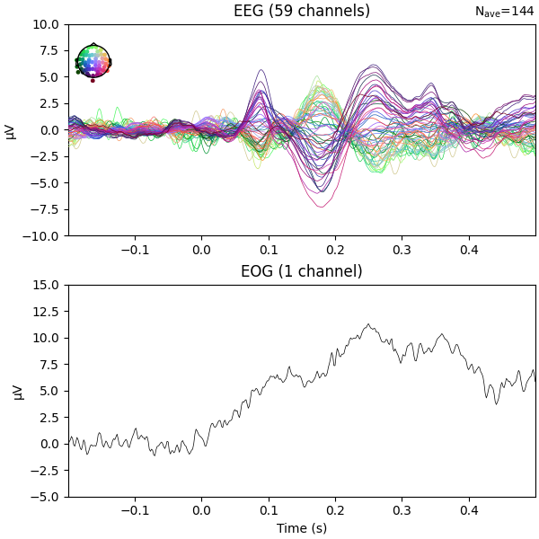
Subtracting Evoked from Epochs
    The following channels are not included in the subtraction: STI 014, EOG 061, STI 016, STI 003, STI 015, STI 001, STI 002, STI 005, STI 006, STI 004
[done]
No projector specified for this dataset. Please consider the method self.add_proj.
No projector specified for this dataset. Please consider the method self.add_proj.
Applying baseline correction (mode: mean)

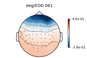
可以看到，即使从 epochs 中去除了诱发响应，我们得到的回归系数仍然相同。

回归前创建 EOG 诱发响应#

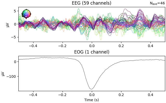
在包含大量 EOG 活动的数据段上估计回归系数更为有利。由于 EOG 活动通常远大于 EEG，EOG 伪迹将在信号中占主导地位，回归系数将主要反映 EOG 的影响。为了增强这一效果，Croft & Barry (2000) [ 2 ] 建议基于眨眼起始点创建 epochs，并计算眨眼的诱发响应。平均过程会抑制与眨眼响应不严格时间锁定的 EEG 信号。理想情况下，应分别为眨眼和扫视创建诱发响应，并建立两个独立的回归模型。不过，我们这里只使用眨眼 epochs，因为 MNE-Python 内置了自动创建眨眼 epochs 的方法。

注意

这与 SSP 采取的方法非常相似。区别在于：SSP 估计与伪迹最大相关的信号成分，并沿该成分去除数据（从而降低非 EOG 数据的秩）；而回归方法利用连续的 EOG 信号来确定去除多少数据（因此不一定降低非 EOG 数据的秩）。总体而言，SSP 倾向于去除过多数据，可能连同真实脑信号一起被消除；而回归则倾向于去除不足，导致部分伪迹信号仍残留在数据中。

eog_epochs = mne.preprocessing.create_eog_epochs(raw)
# We need to explicitly specify that we want to average the EOG channel too.
eog_evoked = eog_epochs.average("all")
eog_evoked.plot("all")
fig.set_size_inches(6, 6)

# perform regression on the evoked blink response
model_evoked = EOGRegression(picks="eeg", picks_artifact="eog").fit(eog_evoked)
fig = model_evoked.plot(vlim=(None, 0.4))
fig.set_size_inches(3, 2)

# apply the regression coefficients to the original epochs
epochs_clean_evoked = model_evoked.apply(epochs).apply_baseline()
fig = epochs_clean_evoked.average("all").plot(**plot_kwargs)
fig.set_size_inches(6, 6)

# for good measure, also show the effect on the blink evoked
eog_evoked_clean = model_evoked.apply(eog_evoked)
eog_evoked_clean.apply_baseline()
eog_evoked_clean.plot("all")
fig.set_size_inches(6, 6)

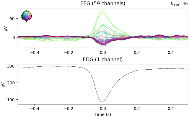
Using EOG channel: EOG 061
EOG channel index for this subject is: [69]
Filtering the data to remove DC offset to help distinguish blinks from saccades
Selecting channel EOG 061 for blink detection
Setting up band-pass filter from 1 - 10 Hz

FIR filter parameters
---------------------
Designing a two-pass forward and reverse, zero-phase, non-causal bandpass filter:
- Windowed frequency-domain design (firwin2) method
- Hann window
- Lower passband edge: 1.00
- Lower transition bandwidth: 0.50 Hz (-12 dB cutoff frequency: 0.75 Hz)
- Upper passband edge: 10.00 Hz
- Upper transition bandwidth: 0.50 Hz (-12 dB cutoff frequency: 10.25 Hz)
- Filter length: 6007 samples (10.001 s)

Now detecting blinks and generating corresponding events
Found 46 significant peaks
Number of EOG events detected: 46
Not setting metadata
46 matching events found
No baseline correction applied
Using data from preloaded Raw for 46 events and 601 original time points ...
0 bad epochs dropped
No projector specified for this dataset. Please consider the method self.add_proj.
No projector specified for this dataset. Please consider the method self.add_proj.
Applying baseline correction (mode: mean)
No projector specified for this dataset. Please consider the method self.add_proj.
Applying baseline correction (mode: mean)

可以看到，回归权重再次得到了正确估计。

可视化对原始数据的处理效果#

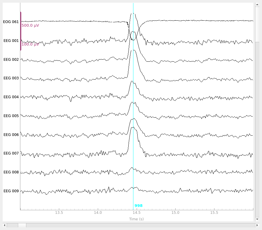
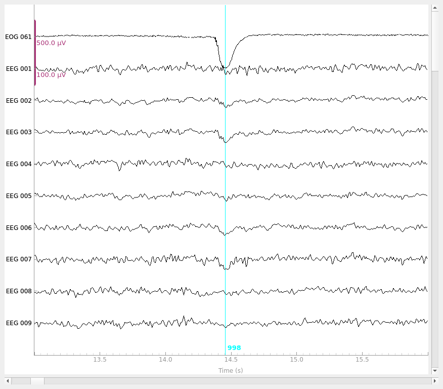
获得稳健的回归权重后，我们可以直接将其应用于 raw、epoched 和 evoked 数据。这里我们使用由眨眼诱发响应得到的回归权重，并将其应用于一个 Raw 实例。

order = np.concatenate(
    [  # plotting order: EOG first, then EEG
        mne.pick_types(raw.info, meg=False, eog=True),
        mne.pick_types(raw.info, meg=False, eeg=True),
    ]
)
raw_kwargs = dict(
    events=eog_epochs.events,
    order=order,
    start=13,
    duration=3,
    n_channels=10,
    scalings=dict(eeg=50e-6, eog=250e-6),
)

# plot original data
raw.plot(**raw_kwargs)

# regress (using coefficients computed previously) and plot
raw_clean = model_evoked.apply(raw)
raw_clean.plot(**raw_kwargs)

No projector specified for this dataset. Please consider the method self.add_proj.

参考文献#

脚本总运行时间：（0 分 4.101 秒）

图库由 Sphinx-Gallery 生成