
非官方中文翻译
本页译自 MNE-Python 官方文档:
查看英文原文 ↗。
文档版权归 MNE Developers 所有(BSD-3-Clause)。
说明
转到末尾下载完整示例代码。
使用等效电流偶极子(ECD)拟合进行源定位#
本教程展示如何使用 MNE-Python 拟合偶极子 [ 1 ]。
如需比较 MNE-C 与 MNE-Python 的拟合结果,请参阅 this gist。
# Authors: The MNE-Python contributors.
# License: BSD-3-Clause
# Copyright the MNE-Python contributors.
import matplotlib.pyplot as plt
import numpy as np
from nilearn.datasets import load_mni152_template
from nilearn.plotting import plot_anat

import mne
from mne.evoked import combine_evoked
from mne.forward import make_forward_dipole
from mne.simulation import simulate_evoked

data_path = mne.datasets.sample.data_path()
subjects_dir = data_path / "subjects"
fname_ave = data_path / "MEG" / "sample" / "sample_audvis-ave.fif"
fname_cov = data_path / "MEG" / "sample" / "sample_audvis-cov.fif"
fname_bem = subjects_dir / "sample" / "bem" / "sample-5120-bem-sol.fif"
fname_trans = data_path / "MEG" / "sample" / "sample_audvis_raw-trans.fif"
fname_surf_lh = subjects_dir / "sample" / "surf" / "lh.white"
让我们定位 N100m(仅使用 MEG)
evoked = mne.read_evokeds(fname_ave, condition="Right Auditory", baseline=(None, 0))
evoked.pick(picks="meg")
evoked_full = evoked.copy()
evoked.crop(0.07, 0.08)

# Fit a dipole
dip = mne.fit_dipole(evoked, fname_cov, fname_bem, fname_trans)[0]

# Plot the result in 3D brain with the MRI image.
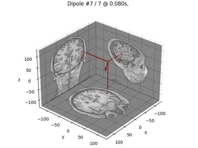
dip.plot_locations(fname_trans, "sample", subjects_dir, mode="orthoview")
Reading /home/circleci/mne_data/MNE-sample-data/MEG/sample/sample_audvis-ave.fif ...
    Read a total of 4 projection items:
        PCA-v1 (1 x 10²) active
        PCA-v2 (1 x 10²) active
        PCA-v3 (1 x 10²) active
        Average EEG reference (1 x 60) active
    Found the data of interest:
        t =    -199.80 ...     499.49 ms (Right Auditory)
        0 CTF compensation matrices available
        nave = 61 - aspect type = 100
Projections have already been applied. Setting proj attribute to True.
Applying baseline correction (mode: mean)
BEM               : PosixPath('/home/circleci/mne_data/MNE-sample-data/subjects/sample/bem/sample-5120-bem-sol.fif')
MRI transform     : /home/circleci/mne_data/MNE-sample-data/MEG/sample/sample_audvis_raw-trans.fif
Head origin       :   -4.2   19.3   65.3 mm rad =   72.3 mm.
Guess grid        :   20.0 mm
Guess mindist     :    5.0 mm
Guess exclude     :   20.0 mm
Using normal MEG coil definitions.
Noise covariance  : /home/circleci/mne_data/MNE-sample-data/MEG/sample/sample_audvis-cov.fif

Coordinate transformation: MRI (surface RAS) -> head
    0.999310 0.009985 -0.035787      -3.17 mm
    0.012759 0.812405 0.582954       6.86 mm
    0.034894 -0.583008 0.811716      28.88 mm
    0.000000 0.000000 0.000000       1.00
Coordinate transformation: MEG device -> head
    0.991420 -0.039936 -0.124467      -6.13 mm
    0.060661 0.984012 0.167456       0.06 mm
    0.115790 -0.173570 0.977991      64.74 mm
    0.000000 0.000000 0.000000       1.00
1 bad channels total
Read 305 MEG channels from info
105 coil definitions read
Coordinate transformation: MEG device -> head
    0.991420 -0.039936 -0.124467      -6.13 mm
    0.060661 0.984012 0.167456       0.06 mm
    0.115790 -0.173570 0.977991      64.74 mm
    0.000000 0.000000 0.000000       1.00
MEG coil definitions created in head coordinates.
Decomposing the sensor noise covariance matrix...
    Created an SSP operator (subspace dimension = 3)
Computing rank from covariance with rank=None
    Using tolerance 3.3e-13 (2.2e-16 eps * 305 dim * 4.8  max singular value)
    Estimated rank (mag + grad): 302
    MEG: rank 302 computed from 305 data channels with 3 projectors
    Setting small MEG eigenvalues to zero (without PCA)
    Created the whitener using a noise covariance matrix with rank 302 (3 small eigenvalues omitted)

---- Computing the forward solution for the guesses...
Guess surface (inner skull) is in MRI (surface RAS) coordinates
Filtering (grid =     20 mm)...
Surface CM = (   0.7  -10.0   44.3) mm
Surface fits inside a sphere with radius   91.8 mm
Surface extent:
    x =  -66.7 ...   68.8 mm
    y =  -88.0 ...   79.0 mm
    z =  -44.5 ...  105.8 mm
Grid extent:
    x =  -80.0 ...   80.0 mm
    y = -100.0 ...   80.0 mm
    z =  -60.0 ...  120.0 mm
900 sources before omitting any.
396 sources after omitting infeasible sources not within 20.0 - 91.8 mm.
Source spaces are in MRI coordinates.
Checking that the sources are inside the surface and at least    5.0 mm away (will take a few...)
Checking surface interior status for 396 points...
    Found  42/396 points inside  an interior sphere of radius   43.6 mm
    Found   0/396 points outside an exterior sphere of radius   91.8 mm
    Found 186/354 points outside using surface Qhull
    Found   9/168 points outside using solid angles
    Total 201/396 points inside the surface
Interior check completed in 11.5 ms
    195 source space points omitted because they are outside the inner skull surface.
    45 source space points omitted because of the    5.0-mm distance limit.
156 sources remaining after excluding the sources outside the surface and less than    5.0 mm inside.
Go through all guess source locations...
[done 156 sources]
---- Fitted :    69.9 ms, distance to inner skull : 10.6868 mm
---- Fitted :    71.6 ms, distance to inner skull : 10.6387 mm
---- Fitted :    73.3 ms, distance to inner skull : 10.5301 mm
---- Fitted :    74.9 ms, distance to inner skull : 10.2493 mm
---- Fitted :    76.6 ms, distance to inner skull : 9.9832 mm
---- Fitted :    78.3 ms, distance to inner skull : 9.7055 mm
---- Fitted :    79.9 ms, distance to inner skull : 9.4112 mm
Projections have already been applied. Setting proj attribute to True.
7 time points fitted
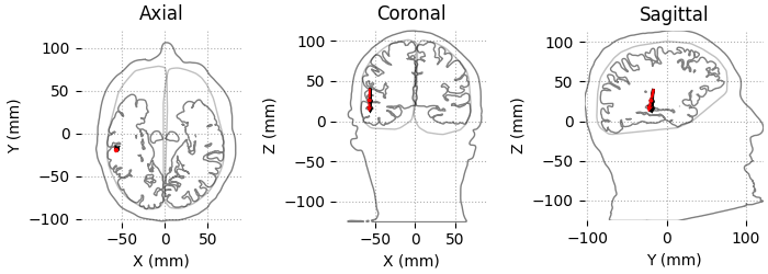
我们还可以使用头部和大脑的轮廓来绘制结果。
color = ["k"] * len(dip)
color[np.argmax(dip.gof)] = "r"
dip.plot_locations(fname_trans, "sample", subjects_dir, mode="outlines", color=color)
Using lh.seghead for head surface.
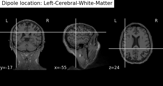
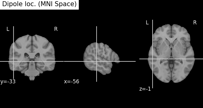
使用 Nilearn 将结果绘制到带有 MRI 图像的 3D 大脑上:分别采用 MRI 坐标和 MNI 坐标(模板大脑)
subject = "sample"
mni_pos = dip.to_mni(subject=subject, trans=fname_trans, subjects_dir=subjects_dir)

mri_pos = dip.to_mri(subject=subject, trans=fname_trans, subjects_dir=subjects_dir)

# Find an anatomical label for the best fitted dipole
best_dip_idx = dip.gof.argmax()
label = dip.to_volume_labels(
    fname_trans, subject=subject, subjects_dir=subjects_dir, aseg="aparc.a2009s+aseg"
)[best_dip_idx]

# Draw dipole position on MRI scan and add anatomical label from parcellation
t1_fname = subjects_dir / subject / "mri" / "T1.mgz"
fig_T1 = plot_anat(t1_fname, cut_coords=mri_pos[0], title=f"Dipole location: {label}")

try:
    template = load_mni152_template(resolution=1)
except TypeError:  # in nilearn < 0.8.1 this did not exist
    template = load_mni152_template()
fig_template = plot_anat(
    template, cut_coords=mni_pos[0], title="Dipole loc. (MNI Space)"
)
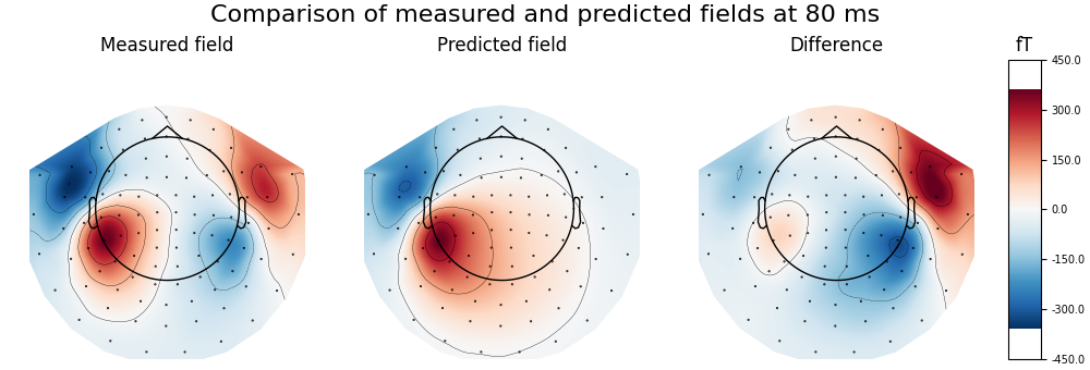
计算并可视化具有最大 GOF 的偶极子所预测的磁场,并与实测数据比较,突出显示同侧(右侧)源
fwd, stc = make_forward_dipole(dip, fname_bem, evoked.info, fname_trans)
pred_evoked = simulate_evoked(fwd, stc, evoked.info, cov=None, nave=np.inf)

# find time point with highest GOF to plot
best_idx = np.argmax(dip.gof)
best_time = dip.times[best_idx]
print(
    f"Highest GOF {dip.gof[best_idx]:0.1f}% at t={best_time * 1000:0.1f} ms with "
    f"confidence volume {dip.conf['vol'][best_idx] * 100**3:0.1f} cm^3"
)
# remember to create a subplot for the colorbar
fig, axes = plt.subplots(
    nrows=1,
    ncols=4,
    figsize=[10.0, 3.4],
    gridspec_kw=dict(width_ratios=[1, 1, 1, 0.1], top=0.85),
    layout="constrained",
)
vmin, vmax = -400, 400  # make sure each plot has same colour range

# first plot the topography at the time of the best fitting (single) dipole
plot_params = dict(times=best_time, ch_type="mag", outlines="head", colorbar=False)
evoked.plot_topomap(time_format="Measured field", axes=axes[0], **plot_params)

# compare this to the predicted field
pred_evoked.plot_topomap(time_format="Predicted field", axes=axes[1], **plot_params)

# Subtract predicted from measured data (apply equal weights)
diff = combine_evoked([evoked, pred_evoked], weights=[1, -1])
plot_params["colorbar"] = True
diff.plot_topomap(time_format="Difference", axes=axes[2:], **plot_params)
fig.suptitle(
    f"Comparison of measured and predicted fields at {best_time * 1000:.0f} ms",
    fontsize=16,
)
Positions (in meters) and orientations
7 sources
Source space          : <SourceSpaces: [<discrete, n_used=7>] head coords, ~3 KiB>
MRI -> head transform : /home/circleci/mne_data/MNE-sample-data/MEG/sample/sample_audvis_raw-trans.fif
Measurement data      : instance of Info
Conductor model   : /home/circleci/mne_data/MNE-sample-data/subjects/sample/bem/sample-5120-bem-sol.fif
Accurate field computations
Do computations in head coordinates
Free source orientations

Read 1 source spaces a total of 7 active source locations

Coordinate transformation: MRI (surface RAS) -> head
    0.999310 0.009985 -0.035787      -3.17 mm
    0.012759 0.812405 0.582954       6.86 mm
    0.034894 -0.583008 0.811716      28.88 mm
    0.000000 0.000000 0.000000       1.00

Read 306 MEG channels from info
105 coil definitions read
Coordinate transformation: MEG device -> head
    0.991420 -0.039936 -0.124467      -6.13 mm
    0.060661 0.984012 0.167456       0.06 mm
    0.115790 -0.173570 0.977991      64.74 mm
    0.000000 0.000000 0.000000       1.00
MEG coil definitions created in head coordinates.
Source spaces are now in head coordinates.

Setting up the BEM model using /home/circleci/mne_data/MNE-sample-data/subjects/sample/bem/sample-5120-bem-sol.fif...

Loading surfaces...

Loading the solution matrix...

Homogeneous model surface loaded.
Loaded linear collocation BEM solution from /home/circleci/mne_data/MNE-sample-data/subjects/sample/bem/sample-5120-bem-sol.fif
Employing the head->MRI coordinate transform with the BEM model.
BEM model sample-5120-bem-sol.fif is now set up


Source spaces are in head coordinates.
Checking that the sources are inside the surface (will take a few...)
Checking surface interior status for 7 points...
    Found 0/7 points inside  an interior sphere of radius   43.6 mm
    Found 0/7 points outside an exterior sphere of radius   91.8 mm
    Found 0/7 points outside using surface Qhull
    Found 0/7 points outside using solid angles
    Total 7/7 points inside the surface
Interior check completed in 1.0 ms
Checking surface interior status for 306 points...
    Found   0/306 points inside  an interior sphere of radius   43.6 mm
    Found 306/306 points outside an exterior sphere of radius   91.8 mm
    Found   0/  0 points outside using surface Qhull
    Found   0/  0 points outside using solid angles
    Total 0/306 points inside the surface
Interior check completed in 0.3 ms

Composing the field computation matrix...
Computing MEG at 7 source locations (free orientations)...

Finished.
    Changing to fixed-orientation forward solution with surface-based source orientations...
    [done]
Projecting source estimate to sensor space...
[done]
Highest GOF 56.9% at t=79.9 ms with confidence volume 8.1 cm^3
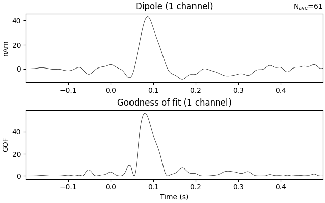
在整个时间区间内估计单个偶极子的时间过程,该偶极子的位置和朝向固定(即使 GOF 最大的那个)
dip_fixed = mne.fit_dipole(
    evoked_full,
    fname_cov,
    fname_bem,
    fname_trans,
    pos=dip.pos[best_idx],
    ori=dip.ori[best_idx],
)[0]
dip_fixed.plot()
BEM               : PosixPath('/home/circleci/mne_data/MNE-sample-data/subjects/sample/bem/sample-5120-bem-sol.fif')
MRI transform     : /home/circleci/mne_data/MNE-sample-data/MEG/sample/sample_audvis_raw-trans.fif
Head origin       :   -4.2   19.3   65.3 mm rad =   72.3 mm.
Fixed position    :  -61.2    5.4   59.6 mm
Fixed orientation  : 0.0099 -0.7504 -0.6609 mm
Noise covariance  : /home/circleci/mne_data/MNE-sample-data/MEG/sample/sample_audvis-cov.fif

Coordinate transformation: MRI (surface RAS) -> head
    0.999310 0.009985 -0.035787      -3.17 mm
    0.012759 0.812405 0.582954       6.86 mm
    0.034894 -0.583008 0.811716      28.88 mm
    0.000000 0.000000 0.000000       1.00
Coordinate transformation: MEG device -> head
    0.991420 -0.039936 -0.124467      -6.13 mm
    0.060661 0.984012 0.167456       0.06 mm
    0.115790 -0.173570 0.977991      64.74 mm
    0.000000 0.000000 0.000000       1.00
1 bad channels total
Read 305 MEG channels from info
105 coil definitions read
Coordinate transformation: MEG device -> head
    0.991420 -0.039936 -0.124467      -6.13 mm
    0.060661 0.984012 0.167456       0.06 mm
    0.115790 -0.173570 0.977991      64.74 mm
    0.000000 0.000000 0.000000       1.00
MEG coil definitions created in head coordinates.
Decomposing the sensor noise covariance matrix...
    Created an SSP operator (subspace dimension = 3)
Computing rank from covariance with rank=None
    Using tolerance 3.3e-13 (2.2e-16 eps * 305 dim * 4.8  max singular value)
    Estimated rank (mag + grad): 302
    MEG: rank 302 computed from 305 data channels with 3 projectors
    Setting small MEG eigenvalues to zero (without PCA)
    Created the whitener using a noise covariance matrix with rank 302 (3 small eigenvalues omitted)
Compute forward for dipole location...
[done 1 source]
Projections have already been applied. Setting proj attribute to True.
421 time points fitted
参考文献#
脚本总运行时间:(0 分钟 9.040 秒)