非官方中文翻译 本页译自 MNE-Python 官方文档： 查看英文原文 ↗。 文档版权归 MNE Developers 所有（BSD-3-Clause）。

显示 EEG 与 MEG 传感器的灵敏度图

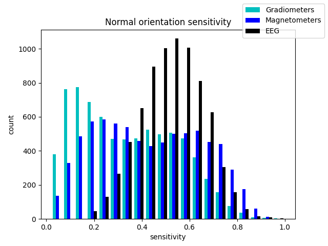
灵敏度图可由正向算子生成，用于指示不同传感器类型探测大脑不同区域神经电流的能力。

如需入门正向建模，请参阅 头模型与正向计算。

# Author: Eric Larson <larson.eric.d@gmail.com>
#
# License: BSD-3-Clause
# Copyright the MNE-Python contributors.

import matplotlib.pyplot as plt
import numpy as np

import mne
from mne.datasets import sample
from mne.source_estimate import SourceEstimate
from mne.source_space import compute_distance_to_sensors

print(__doc__)

data_path = sample.data_path()
meg_path = data_path / "MEG" / "sample"
fwd_fname = meg_path / "sample_audvis-meg-eeg-oct-6-fwd.fif"
subjects_dir = data_path / "subjects"

# Read the forward solutions with surface orientation
fwd = mne.read_forward_solution(fwd_fname)
mne.convert_forward_solution(fwd, surf_ori=True, copy=False)
leadfield = fwd["sol"]["data"]
print("Leadfield shape : {leadfield.shape}")

Reading forward solution from /home/circleci/mne_data/MNE-sample-data/MEG/sample/sample_audvis-meg-eeg-oct-6-fwd.fif...
    Reading a source space...
    Computing patch statistics...
    Patch information added...
    Distance information added...
    [done]
    Reading a source space...
    Computing patch statistics...
    Patch information added...
    Distance information added...
    [done]
    2 source spaces read
    Desired named matrix (kind = 3523 (FIFF_MNE_FORWARD_SOLUTION_GRAD)) not available
    Read MEG forward solution (7498 sources, 306 channels, free orientations)
    Desired named matrix (kind = 3523 (FIFF_MNE_FORWARD_SOLUTION_GRAD)) not available
    Read EEG forward solution (7498 sources, 60 channels, free orientations)
    Forward solutions combined: MEG, EEG
    Source spaces transformed to the forward solution coordinate frame
    Average patch normals will be employed in the rotation to the local surface coordinates....
    Converting to surface-based source orientations...
    [done]
Leadfield shape : {leadfield.shape}

计算灵敏度图

grad_map = mne.sensitivity_map(fwd, ch_type="grad", mode="fixed")
mag_map = mne.sensitivity_map(fwd, ch_type="mag", mode="fixed")
eeg_map = mne.sensitivity_map(fwd, ch_type="eeg", mode="fixed")

    204 out of 366 channels remain after picking
    102 out of 366 channels remain after picking
    60 out of 366 channels remain after picking
Adding average EEG reference projection.

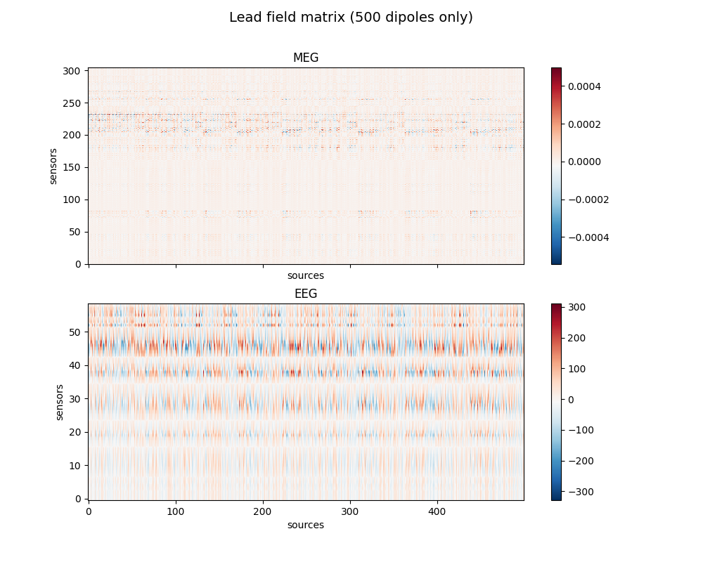
结合灵敏度图显示增益矩阵（又称导联场矩阵）

picks_meg = mne.pick_types(fwd["info"], meg=True, eeg=False)
picks_eeg = mne.pick_types(fwd["info"], meg=False, eeg=True)

fig, axes = plt.subplots(2, 1, figsize=(10, 8), sharex=True)
fig.suptitle("Lead field matrix (500 dipoles only)", fontsize=14)
for ax, picks, ch_type in zip(axes, [picks_meg, picks_eeg], ["meg", "eeg"]):
    im = ax.imshow(leadfield[picks, :500], origin="lower", aspect="auto", cmap="RdBu_r")
    ax.set_title(ch_type.upper())
    ax.set_xlabel("sources")
    ax.set_ylabel("sensors")
    fig.colorbar(im, ax=ax)

fig_2, ax = plt.subplots()
ax.hist(
    [grad_map.data.ravel(), mag_map.data.ravel(), eeg_map.data.ravel()],
    bins=20,
    label=["Gradiometers", "Magnetometers", "EEG"],
    color=["c", "b", "k"],
)
fig_2.legend()
ax.set(title="Normal orientation sensitivity", xlabel="sensitivity", ylabel="count")

brain_sens = grad_map.plot(
    subjects_dir=subjects_dir, clim=dict(lims=[0, 50, 100]), figure=1
)
brain_sens.add_text(0.1, 0.9, "Gradiometer sensitivity", "title", font_size=16)

• 
• 

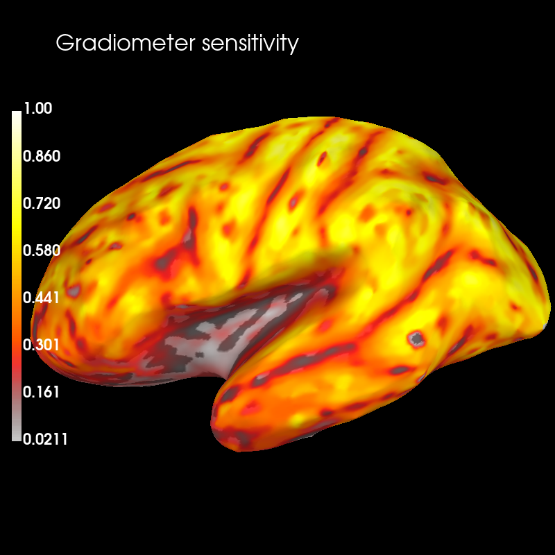
Using control points [0.02108201 0.32186553 1.        ]

比较灵敏度图与源深度分布

# source space with vertices
src = fwd["src"]

# Compute minimum Euclidean distances between vertices and MEG sensors
depths = compute_distance_to_sensors(src=src, info=fwd["info"], picks=picks_meg).min(
    axis=1
)
maxdep = depths.max()  # for scaling

vertices = [src[0]["vertno"], src[1]["vertno"]]

depths_map = SourceEstimate(data=depths, vertices=vertices, tmin=0.0, tstep=1.0)

brain_dep = depths_map.plot(
    subject="sample",
    subjects_dir=subjects_dir,
    clim=dict(kind="value", lims=[0, maxdep / 2.0, maxdep]),
    figure=2,
)
brain_dep.add_text(0.1, 0.9, "Source depth (m)", "title", font_size=16)

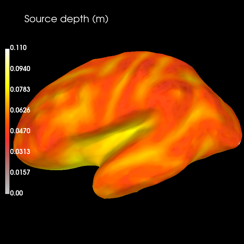
灵敏度很可能与源到传感器之间的距离共同变化。为确定这种关系的强度，我们可以计算源深度与灵敏度值之间的相关性。

corr = np.corrcoef(depths, grad_map.data[:, 0])[0, 1]
print(f"Correlation between source depth and gradiomter sensitivity values: {corr:f}.")

Correlation between source depth and gradiomter sensitivity values: -0.815476.

梯度计的灵敏度在靠近传感器处最高，并随源深度增加而迅速下降。两者之间高度的负相关证实了这一点。