非官方中文翻译本页译自 MNE-Python 官方文档：查看英文原文 ↗。文档版权归 MNE Developers 所有（BSD-3-Clause）。

说明

转到末尾下载完整示例代码。

使用受试者解剖结构模拟原始数据#

本示例说明如何使用 mne.simulation.SourceSimulator 类结合受试者解剖结构生成源估计并模拟原始数据。模拟出原始数据后，再用动态统计参数映射（dSPM）逆算子重建源估计。

# Author: Ivana Kojcic <ivana.kojcic@gmail.com>
#         Eric Larson <larson.eric.d@gmail.com>
#         Kostiantyn Maksymenko <kostiantyn.maksymenko@gmail.com>
#         Samuel Deslauriers-Gauthier <sam.deslauriers@gmail.com>

# License: BSD-3-Clause
# Copyright the MNE-Python contributors.

import numpy as np

import mne
from mne.datasets import sample

本示例将为示例受试者模拟原始数据，因此需要加载其信息。若本机尚无数据，这一步会自动下载；同时设置受试者目录，避免每次调用函数时重复传入。

data_path = sample.data_path()
subjects_dir = data_path / "subjects"
subject = "sample"
meg_path = data_path / "MEG" / subject

首先，从示例受试者获取 info 结构。

fname_info = meg_path / "sample_audvis_raw.fif"
info = mne.io.read_info(fname_info)
tstep = 1 / info["sfreq"]

Read a total of 3 projection items:
    PCA-v1 (1 x 102)  idle
    PCA-v2 (1 x 102)  idle
    PCA-v3 (1 x 102)  idle

模拟源还需要源空间，可从示例受试者的正向解中获得。

fwd_fname = meg_path / "sample_audvis-meg-eeg-oct-6-fwd.fif"
fwd = mne.read_forward_solution(fwd_fname)
src = fwd["src"]

Reading forward solution from /home/circleci/mne_data/MNE-sample-data/MEG/sample/sample_audvis-meg-eeg-oct-6-fwd.fif...
    Reading a source space...
    Computing patch statistics...
    Patch information added...
    Distance information added...
    [done]
    Reading a source space...
    Computing patch statistics...
    Patch information added...
    Distance information added...
    [done]
    2 source spaces read
    Desired named matrix (kind = 3523 (FIFF_MNE_FORWARD_SOLUTION_GRAD)) not available
    Read MEG forward solution (7498 sources, 306 channels, free orientations)
    Desired named matrix (kind = 3523 (FIFF_MNE_FORWARD_SOLUTION_GRAD)) not available
    Read EEG forward solution (7498 sources, 60 channels, free orientations)
    Forward solutions combined: MEG, EEG
    Source spaces transformed to the forward solution coordinate frame

模拟原始数据需要用事件矩阵定义活动发生的时间，并指定各事件的 ID；此外还需定义噪声协方差矩阵。这里两者都从示例数据集加载，用户也可以自行指定。

fname_event = meg_path / "sample_audvis_raw-eve.fif"
fname_cov = meg_path / "sample_audvis-cov.fif"

events = mne.read_events(fname_event)
noise_cov = mne.read_cov(fname_cov)

# Standard sample event IDs. These values will correspond to the third column
# in the events matrix.
event_id = {
    "auditory/left": 1,
    "auditory/right": 2,
    "visual/left": 3,
    "visual/right": 4,
    "smiley": 5,
    "button": 32,
}


# Take only a few events for speed
events = events[:80]

366 x 366 full covariance (kind = 1) found.
Read a total of 4 projection items:
    PCA-v1 (1 x 102) active
    PCA-v2 (1 x 102) active
    PCA-v3 (1 x 102) active
    Average EEG reference (1 x 60) active

为了模拟源时间过程，需要为 4 个模拟条件分别指定目标激活区域的标签。构建一个字典，把各条件映射到 aparc.a2009s [1] 标签内的激活强度。在 aparc.a2009s 分区中：

‘G_temp_sup-G_T_transv’ 是初级听觉区的标签
‘S_calcarine’ 是初级视觉区的标签

在 4 个条件中，每次只激活初级区域。也就是说，听觉区激活时视觉区不激活，反之亦然。此外，每个条件下对侧区域的活动强于同侧区域（此处为 2 倍）。

activations = {
    "auditory/left": [
        ("G_temp_sup-G_T_transv-lh", 30),  # label, activation (nAm)
        ("G_temp_sup-G_T_transv-rh", 60),
    ],
    "auditory/right": [
        ("G_temp_sup-G_T_transv-lh", 60),
        ("G_temp_sup-G_T_transv-rh", 30),
    ],
    "visual/left": [("S_calcarine-lh", 30), ("S_calcarine-rh", 60)],
    "visual/right": [("S_calcarine-lh", 60), ("S_calcarine-rh", 30)],
}

annot = "aparc.a2009s"

# Load the 4 necessary label names.
label_names = sorted(
    set(
        activation[0]
        for activation_list in activations.values()
        for activation in activation_list
    )
)
region_names = list(activations.keys())

创建模拟的源活动#

为每个区域生成源时间过程。本示例一次只模拟一个条件的源活动，因此每个诱发响应由潜伏期与持续时间参数化。

def data_fun(times, latency, duration):
    """Generate source time courses for evoked responses."""
    f = 15  # oscillating frequency, beta band [Hz]
    sigma = 0.375 * duration
    sinusoid = np.sin(2 * np.pi * f * (times - latency))
    gf = np.exp(
        -((times - latency - rng.uniform(high=sigma / 4.0, size=1)) ** 2)
        / (2 * (sigma**2))
    )
    return 1e-9 * sinusoid * gf

这里使用 SourceSimulator，它可以指定事件类型发生的位置（label）、内容（source_time_series）与时间（events）。

我们将为 4 个区域添加数据，每个区域包含 2 个标签。由于 add_data 方法每次只接受 1 个标签，因此每个区域需调用 2 次。

生成的诱发响应主成分在 100 ms 处达到峰值，持续约 30 ms，首先出现在对侧皮层；随后同侧皮层出现响应，峰值约晚 15 ms。如前所述，对侧区域的激活幅度为同侧的 2 倍。

活动发生的时间由事件定义。这里的事件取自原始数据：第一列是事件所在的采样点，第二列不使用，第三列是事件 ID，4 个区域各不相同。

times = np.arange(150, dtype=np.float64) / info["sfreq"]
duration = 0.03
rng = np.random.default_rng(7)
source_simulator = mne.simulation.SourceSimulator(src, tstep=tstep)

for region_id, region_name in enumerate(region_names, 1):
    events_tmp = events[np.where(events[:, 2] == region_id)[0], :]
    for i in range(2):
        label_name = activations[region_name][i][0]
        label_tmp = mne.read_labels_from_annot(
            subject, annot, subjects_dir=subjects_dir, regexp=label_name, verbose=False
        )
        label_tmp = label_tmp[0]
        amplitude_tmp = activations[region_name][i][1]
        if region_name.split("/")[1][0] == label_tmp.hemi[0]:
            latency_tmp = 0.115
        else:
            latency_tmp = 0.1
        wf_tmp = data_fun(times, latency_tmp, duration)
        source_simulator.add_data(label_tmp, amplitude_tmp * wf_tmp, events_tmp)

# To obtain a SourceEstimate object, we need to use `get_stc()` method of
# SourceSimulator class.
stc_data = source_simulator.get_stc()

模拟原始数据#

把源时间序列投影到传感器空间，并向模拟原始数据加入三类噪声：

由示例数据噪声协方差得到的多变量高斯噪声
眨眼（EOG）噪声
ECG 噪声

SourceSimulator 可以直接传给 simulate_raw() 函数。

raw_sim = mne.simulation.simulate_raw(info, source_simulator, forward=fwd)
raw_sim.set_eeg_reference(projection=True)

mne.simulation.add_noise(raw_sim, cov=noise_cov, rng=211)
mne.simulation.add_eog(raw_sim, rng=223)
mne.simulation.add_ecg(raw_sim, rng=227)

# Plot original and simulated raw data.
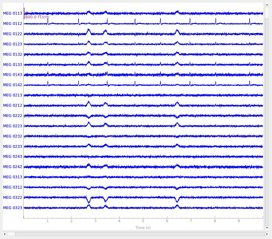
raw_sim.plot(title="Simulated raw data")

Setting up raw simulation: 1 position, "cos2" interpolation
Event information stored on channel:              STI 014
    Interval 0.000–1.665 s
Setting up forward solutions
Computing gain matrix for transform #1/1
    Interval 0.000–1.665 s
    Interval 0.000–1.665 s
    Interval 0.000–1.665 s
    Interval 0.000–1.665 s
    Interval 0.000–1.665 s
    Interval 0.000–1.665 s
    Interval 0.000–1.665 s
    Interval 0.000–1.665 s
    Interval 0.000–1.665 s
    Interval 0.000–1.665 s
    Interval 0.000–1.665 s
    Interval 0.000–1.665 s
    Interval 0.000–1.665 s
    Interval 0.000–1.665 s
    Interval 0.000–1.665 s
    Interval 0.000–1.665 s
    Interval 0.000–1.665 s
    Interval 0.000–1.665 s
    Interval 0.000–1.665 s
    Interval 0.000–1.665 s
    Interval 0.000–1.665 s
    Interval 0.000–1.665 s
    Interval 0.000–1.665 s
    Interval 0.000–1.665 s
    Interval 0.000–1.665 s
    Interval 0.000–1.665 s
    Interval 0.000–1.665 s
    Interval 0.000–1.665 s
    Interval 0.000–1.665 s
    Interval 0.000–1.665 s
    Interval 0.000–1.665 s
    Interval 0.000–1.665 s
    Interval 0.000–1.665 s
    Interval 0.000–1.665 s
    Interval 0.000–1.665 s
    Interval 0.000–1.665 s
    Interval 0.000–1.665 s
    Interval 0.000–1.665 s
    Interval 0.000–1.665 s
    Interval 0.000–1.665 s
    Interval 0.000–1.665 s
    Interval 0.000–1.665 s
    Interval 0.000–1.665 s
    Interval 0.000–1.665 s
    Interval 0.000–1.665 s
    Interval 0.000–1.665 s
    Interval 0.000–1.665 s
    Interval 0.000–1.665 s
    Interval 0.000–1.665 s
    Interval 0.000–1.665 s
    Interval 0.000–1.665 s
    Interval 0.000–1.665 s
    Interval 0.000–1.665 s
    Interval 0.000–1.665 s
    Interval 0.000–1.665 s
    Interval 0.000–1.665 s
    Interval 0.000–1.665 s
    Interval 0.000–1.665 s
    Interval 0.000–0.105 s
    60 STC iterations provided
[done]
EEG channel type selected for re-referencing
Adding average EEG reference projection.
1 projection items deactivated
Average reference projection was added, but has not been applied yet. Use the apply_proj method to apply it.
Adding noise to 366/376 channels (366 channels in cov)
Sphere                : origin at (0.0 0.0 0.0) mm
              radius  : 0.1 mm
Source location file  : dict()
Assuming input in millimeters
Assuming input in MRI coordinates

Positions (in meters) and orientations
2 sources
blink simulated and trace stored on channel:      EOG 061
Setting up forward solutions
Computing gain matrix for transform #1/1
Sphere                : origin at (0.0 0.0 0.0) mm
              radius  : 0.1 mm
Source location file  : dict()
Assuming input in millimeters
Assuming input in MRI coordinates

Positions (in meters) and orientations
1 sources
ecg simulated and trace not stored
Setting up forward solutions
Computing gain matrix for transform #1/1

提取分段并计算诱发响应#

epochs = mne.Epochs(
    raw_sim,
    events,
    event_id,
    tmin=-0.2,
    tmax=0.3,
    baseline=(None, 0),
    on_outside="ignore",
)
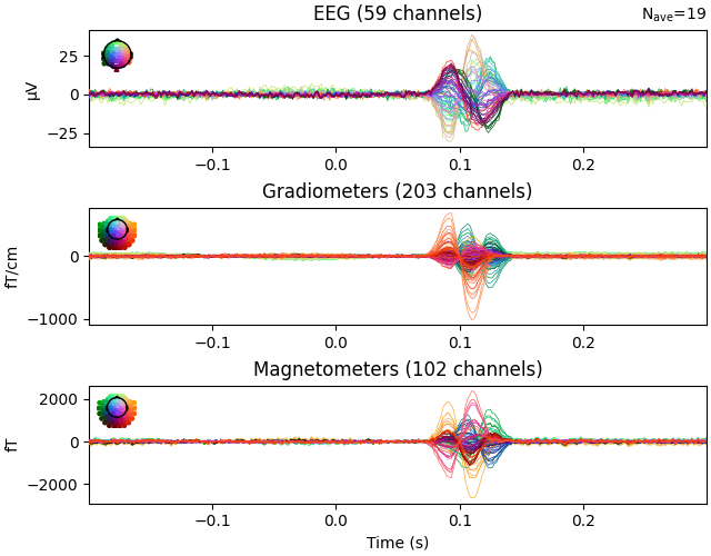
evoked_aud_left = epochs["auditory/left"].average()
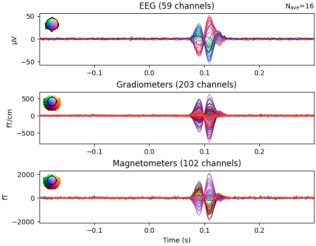
evoked_vis_right = epochs["visual/right"].average()

# Visualize the evoked data
evoked_aud_left.plot(spatial_colors=True)
evoked_vis_right.plot(spatial_colors=True)

Not setting metadata
80 matching events found
Setting baseline interval to [-0.19979521315838786, 0.0] s
Applying baseline correction (mode: mean)
Created an SSP operator (subspace dimension = 4)
4 projection items activated

使用 dSPM 逆算子重建模拟的源时间过程#

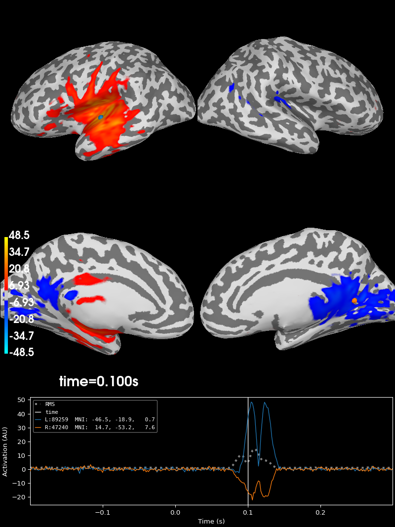
这里分别重建听觉区与视觉区的源时间过程，并展示二者之差，只是为了更直观地呈现源重建结果。正如预期，初级听觉区出现强激活时，初级视觉区激活较弱，反之亦然。

method, lambda2 = "dSPM", 1.0 / 9.0
inv = mne.minimum_norm.make_inverse_operator(epochs.info, fwd, noise_cov)
stc_aud = mne.minimum_norm.apply_inverse(evoked_aud_left, inv, lambda2, method)
stc_vis = mne.minimum_norm.apply_inverse(evoked_vis_right, inv, lambda2, method)
stc_diff = stc_aud - stc_vis

brain = stc_diff.plot(
    subjects_dir=subjects_dir, initial_time=0.1, hemi="split", views=["lat", "med"]
)

simulated raw data using subject anatomy

Converting forward solution to surface orientation
    Average patch normals will be employed in the rotation to the local surface coordinates....
    Converting to surface-based source orientations...
    [done]
Computing inverse operator with 364 channels.
    364 out of 366 channels remain after picking
Selected 364 channels
Creating the depth weighting matrix...
    203 planar channels
    limit = 7262/7498 = 10.020865
    scale = 2.58122e-08 exp = 0.8
Applying loose dipole orientations to surface source spaces: 0.2
Whitening the forward solution.
    Created an SSP operator (subspace dimension = 4)
Computing rank from covariance with rank=None
    Using tolerance 3.3e-13 (2.2e-16 eps * 305 dim * 4.8  max singular value)
    Estimated rank (mag + grad): 302
    MEG: rank 302 computed from 305 data channels with 3 projectors
    Using tolerance 4.7e-14 (2.2e-16 eps * 59 dim * 3.6  max singular value)
    Estimated rank (eeg): 58
    EEG: rank 58 computed from 59 data channels with 1 projector
    Setting small MEG eigenvalues to zero (without PCA)
    Setting small EEG eigenvalues to zero (without PCA)
Creating the source covariance matrix
Adjusting source covariance matrix.
Computing SVD of whitened and weighted lead field matrix.
    largest singular value = 5.49264
    scaling factor to adjust the trace = 1.64e+19 (nchan = 364 nzero = 4)
Preparing the inverse operator for use...
    Scaled noise and source covariance from nave = 1 to nave = 19
    Created the regularized inverter
    Created an SSP operator (subspace dimension = 4)
    Created the whitener using a noise covariance matrix with rank 360 (4 small eigenvalues omitted)
    Computing noise-normalization factors (dSPM)...
[done]
Applying inverse operator to "auditory/left"...
    Picked 364 channels from the data
    Computing inverse...
    Eigenleads need to be weighted ...
    Computing residual...
    Explained  87.0% variance
    Combining the current components...
    dSPM...
[done]
Preparing the inverse operator for use...
    Scaled noise and source covariance from nave = 1 to nave = 16
    Created the regularized inverter
    Created an SSP operator (subspace dimension = 4)
    Created the whitener using a noise covariance matrix with rank 360 (4 small eigenvalues omitted)
    Computing noise-normalization factors (dSPM)...
[done]
Applying inverse operator to "visual/right"...
    Picked 364 channels from the data
    Computing inverse...
    Eigenleads need to be weighted ...
    Computing residual...
    Explained  90.9% variance
    Combining the current components...
    dSPM...
[done]
Using control points [ 3.20599217  4.81842689 48.67130457]

参考文献#

脚本总运行时间：（0 分 13.847 秒）

图库由 Sphinx-Gallery 生成