
说明
转到末尾下载完整示例代码。
处理 CTF 数据:Brainstorm 听觉数据集#
这里我们针对 Brainstorm 听觉教程数据集,从原始数据计算诱发响应。作为对比,请参见 [1] 以及相关的 brainstorm 网站。
实验:
一名被试,2 次采集运行,每次 6 分钟。
每次运行包含 200 个标准蜂鸣声和 40 个明显偏差的蜂鸣声。
随机 ISI:在 0.7 秒到 1.7 秒之间均匀分布。
检测到偏差刺激时用右手食指按键。
# Authors: Mainak Jas <mainak.jas@telecom-paristech.fr>
#          Eric Larson <larson.eric.d@gmail.com>
#          Jaakko Leppakangas <jaeilepp@student.jyu.fi>
#
# License: BSD-3-Clause
# Copyright the MNE-Python contributors.
import numpy as np
import pandas as pd

import mne
from mne import combine_evoked
from mne.datasets.brainstorm import bst_auditory
from mne.io import read_raw_ctf
from mne.minimum_norm import apply_inverse
为减少内存消耗和运行时间,部分步骤已预先计算。若要从头运行全部流程,请将 use_precomputed 改为 False。当 use_precomputed = False 时,即使在性能较好的计算机上,本脚本的运行时间也可能达到数分钟。
use_precomputed = True
数据由 CTF 275 系统以 2400 Hz 采集,并在 600 Hz 处进行低通滤波。这里读取数据和空房间数据文件,以构建 mne.io.Raw 实例。
data_path = bst_auditory.data_path()

subject = "bst_auditory"
subjects_dir = data_path / "subjects"

raw_fname1 = data_path / "MEG" / subject / "S01_AEF_20131218_01.ds"
raw_fname2 = data_path / "MEG" / subject / "S01_AEF_20131218_02.ds"
erm_fname = data_path / "MEG" / subject / "S01_Noise_20131218_01.ds"
在节省内存模式下,我们使用 preload=False,并采用按需加载数据的高效 IO。不过,滤波及其他一些函数需要先将数据预加载到内存中。
raw = read_raw_ctf(raw_fname1)
n_times_run1 = raw.n_times

# Here we ignore that these have different device<->head transforms
mne.io.concatenate_raws([raw, read_raw_ctf(raw_fname2)], on_mismatch="ignore")
raw_erm = read_raw_ctf(erm_fname)
ds directory : /home/circleci/mne_data/MNE-brainstorm-data/bst_auditory/MEG/bst_auditory/S01_AEF_20131218_01.ds
    res4 data read.
    hc data read.
    Separate EEG position data file read.
    Quaternion matching (desired vs. transformed):
       2.51   74.26    0.00 mm <->    2.51   74.26   -0.00 mm (orig :  -56.69   50.20 -264.38 mm) diff =    0.000 mm
      -2.51  -74.26    0.00 mm <->   -2.51  -74.26   -0.00 mm (orig :   50.89  -52.31 -265.88 mm) diff =    0.000 mm
     108.63    0.00    0.00 mm <->  108.63    0.00    0.00 mm (orig :   67.41   77.68 -239.53 mm) diff =    0.000 mm
    Coordinate transformations established.
    Reading digitizer points from ['/home/circleci/mne_data/MNE-brainstorm-data/bst_auditory/MEG/bst_auditory/S01_AEF_20131218_01.ds/S01_20131218_01.pos']...
    Polhemus data for 3 HPI coils added
    Device coordinate locations for 3 HPI coils added
    5 extra points added to Polhemus data.
    Measurement info composed.
Finding samples for /home/circleci/mne_data/MNE-brainstorm-data/bst_auditory/MEG/bst_auditory/S01_AEF_20131218_01.ds/S01_AEF_20131218_01.meg4:
    System clock channel is available, checking which samples are valid.
    360 x 2400 = 864000 samples from 340 chs
Current compensation grade : 3
ds directory : /home/circleci/mne_data/MNE-brainstorm-data/bst_auditory/MEG/bst_auditory/S01_AEF_20131218_02.ds
    res4 data read.
    hc data read.
    Separate EEG position data file read.
    Quaternion matching (desired vs. transformed):
       2.64   74.60    0.00 mm <->    2.64   74.60   -0.00 mm (orig :  -58.07   49.23 -263.11 mm) diff =    0.000 mm
      -2.64  -74.60    0.00 mm <->   -2.64  -74.60   -0.00 mm (orig :   49.94  -53.82 -265.07 mm) diff =    0.000 mm
     108.24    0.00    0.00 mm <->  108.24   -0.00    0.00 mm (orig :   66.67   76.99 -243.39 mm) diff =    0.000 mm
    Coordinate transformations established.
    Reading digitizer points from ['/home/circleci/mne_data/MNE-brainstorm-data/bst_auditory/MEG/bst_auditory/S01_AEF_20131218_02.ds/S01_20131218_01.pos']...
    Polhemus data for 3 HPI coils added
    Device coordinate locations for 3 HPI coils added
    5 extra points added to Polhemus data.
    Measurement info composed.
Finding samples for /home/circleci/mne_data/MNE-brainstorm-data/bst_auditory/MEG/bst_auditory/S01_AEF_20131218_02.ds/S01_AEF_20131218_02.meg4:
    System clock channel is available, checking which samples are valid.
    360 x 2400 = 864000 samples from 340 chs
Current compensation grade : 3
ds directory : /home/circleci/mne_data/MNE-brainstorm-data/bst_auditory/MEG/bst_auditory/S01_Noise_20131218_01.ds
    res4 data read.
    hc data read.
    Separate EEG position data file read.
    Quaternion matching (desired vs. transformed):
       0.00   80.00    0.00 mm <->    0.00   80.00    0.00 mm (orig :  -56.57   56.57 -270.00 mm) diff =    0.000 mm
       0.00  -80.00    0.00 mm <->    0.00  -80.00    0.00 mm (orig :   56.57  -56.57 -270.00 mm) diff =    0.000 mm
      80.00    0.00    0.00 mm <->   80.00   -0.00    0.00 mm (orig :   56.57   56.57 -270.00 mm) diff =    0.000 mm
    Coordinate transformations established.
    Polhemus data for 3 HPI coils added
    Device coordinate locations for 3 HPI coils added
    Measurement info composed.
Finding samples for /home/circleci/mne_data/MNE-brainstorm-data/bst_auditory/MEG/bst_auditory/S01_Noise_20131218_01.ds/S01_Noise_20131218_01.meg4:
    System clock channel is available, checking which samples are valid.
    15 x 4800 = 72000 samples from 301 chs
Current compensation grade : 3
数据数组包含 274 个 MEG 轴向梯度计、26 个 MEG 参考传感器和 2 个 EEG 电极(Cz 和 Pz)。此外:
1 个 stim 通道,用于标记刺激的呈现时间
1 个音频通道,用于记录发送的信号
1 个反应通道,用于记录按键
1 个双极 ECG 通道
2 个双极 EOG 通道(垂直和水平)
12 个头位跟踪通道
20 个未使用通道
另请注意,数字化电极位置(存储在 .pos 文件中)已被自动加载并添加到 Raw 对象。
头位跟踪通道和未使用通道被标记为 misc 通道。这里我们定义 EOG 和 ECG 通道。
raw.set_channel_types({"HEOG": "eog", "VEOG": "eog", "ECG": "ecg"})
if not use_precomputed:
    # Leave out the two EEG channels for easier computation of forward.
    raw.pick(["meg", "stim", "misc", "eog", "ecg"]).load_data()
为降低噪声,我们识别出一组坏段并存储在 csv 文件中。随后利用这些坏段剔除与其重叠的 epoch。第二次运行的文件中还包含一些扫视。扫视通过 SSP 去除。我们使用 pandas 从 csv 文件中读取数据。你也可以用自己喜欢的文本编辑器查看这些文件。
annotations_df = pd.DataFrame()
offset = n_times_run1
for idx in [1, 2]:
    csv_fname = data_path / "MEG" / "bst_auditory" / f"events_bad_0{idx}.csv"
    df = pd.read_csv(csv_fname, header=None, names=["onset", "duration", "id", "label"])
    print(f"Events from run {idx}:")
    print(df)

    df["onset"] += offset * (idx - 1)
    annotations_df = pd.concat([annotations_df, df], axis=0)

saccades_events = df[df["label"] == "saccade"].values[:, :3].astype(int)

# Conversion from samples to times:
onsets = annotations_df["onset"].values / raw.info["sfreq"]
durations = annotations_df["duration"].values / raw.info["sfreq"]
descriptions = annotations_df["label"].values

annotations = mne.Annotations(onsets, durations, descriptions)
raw.set_annotations(annotations)
del onsets, durations, descriptions
Events from run 1:
     onset  duration  id label
0     7625      2776   1   BAD
1   142459       892   1   BAD
2   216954       460   1   BAD
3   345135      5816   1   BAD
4   357687      1053   1   BAD
5   409101      3736   1   BAD
6   461110       179   1   BAD
7   479866       426   1   BAD
8   764914     11500   1   BAD
9   798174      6589   1   BAD
10  846880      5383   1   BAD
11  858863      5136   1   BAD
Events from run 2:
     onset  duration  id    label
0        9      5583   1      BAD
1     9256      3114   1      BAD
2    14287      3456   1      BAD
3   116432       228   1      BAD
4   134489      1329   1      BAD
5   464527      4727   1      BAD
6   494136      4519   1      BAD
7   749288       189   1      BAD
8   788623      7937   1      BAD
9    21179         0   1  saccade
10   72993         0   1  saccade
11  134527         0   1  saccade
12  196555         0   1  saccade
13  249894         0   1  saccade
14  343357         0   1  saccade
15  400771         0   1  saccade
16  450256         0   1  saccade
17  593101         0   1  saccade
18  733942         0   1  saccade
19  765939         0   1  saccade
20  789476         0   1  saccade
21  792852         0   1  saccade
22  833208         0   1  saccade
23  859869         0   1  saccade
24  862888         0   1  saccade
这里我们为磁强计计算扫视和 EOG 投影器,并将它们添加到原始数据中。投影器会被添加到两次运行的数据中。
saccade_epochs = mne.Epochs(
    raw,
    saccades_events,
    1,
    0.0,
    0.5,
    preload=True,
    baseline=(None, None),
    reject_by_annotation=False,
)

projs_saccade = mne.compute_proj_epochs(
    saccade_epochs, n_mag=1, n_eeg=0, desc_prefix="saccade"
)
if use_precomputed:
    proj_fname = data_path / "MEG" / "bst_auditory" / "bst_auditory-eog-proj.fif"
    projs_eog = mne.read_proj(proj_fname)[0]
else:
    projs_eog, _ = mne.preprocessing.compute_proj_eog(raw.load_data(), n_mag=1, n_eeg=0)
raw.add_proj(projs_saccade)
raw.add_proj(projs_eog)
del saccade_epochs, saccades_events, projs_eog, projs_saccade  # To save memory
Not setting metadata
16 matching events found
Setting baseline interval to [0.0, 0.5] s
Applying baseline correction (mode: mean)
0 projection items activated
Loading data for 16 events and 1201 original time points ...
1 bad epochs dropped
No channels 'grad' found. Skipping.
Adding projection: axial-saccade-PCA-01 (exp var=38.1%)
    Read a total of 1 projection items:
        EOG-axial-998--0.200-0.200-PCA-01 (1 x 274)  idle
1 projection items deactivated
1 projection items deactivated
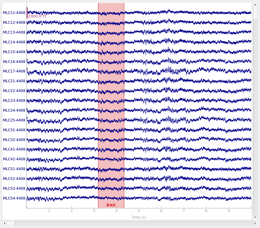
目视检查投影的效果。点击右下角的“proj”按钮可切换投影器的开启/关闭。将事件列表作为关键字参数传入即可绘制 EOG 事件。由于坏段和扫视已作为标注添加到原始数据中,它们也会被绘制出来。
raw.plot()
Using qt as 2D backend.
典型的预处理步骤是去除工频伪迹(50 Hz 或 60 Hz)。这里我们在 60、120 和 180 Hz 处对数据进行陷波滤波,以去除原始的 60 Hz 伪迹及其谐波。图中绘制了滤波前后的功率谱以展示效果。600 Hz 之后的下降是因为数据在采集期间已被滤波。在节省内存模式下,我们在诱发阶段进行滤波,这通常并不是你会采用的做法。
if not use_precomputed:
    raw.compute_psd(tmax=np.inf, picks="meg").plot(
        picks="data", exclude="bads", amplitude=False
    )
    notches = np.arange(60, 181, 60)
    raw.notch_filter(notches, phase="zero-double", fir_design="firwin2")
    raw.compute_psd(tmax=np.inf, picks="meg").plot(
        picks="data", exclude="bads", amplitude=False
    )
我们还会在 100 Hz 处对数据进行低通滤波,以去除高频成分。
if not use_precomputed:
    raw.filter(
        None,
        100.0,
        h_trans_bandwidth=0.5,
        filter_length="10s",
        phase="zero-double",
        fir_design="firwin2",
    )
分段与平均。首先定义一些参数,并从刺激通道(UPPT001)中提取事件。剔除阈值以峰峰值定义,梯度计单位为 T/m,磁强计单位为 T,EOG 和 EEG 通道单位为 V。
Finding events on: UPPT001
480 events found on stim channel UPPT001
Event IDs: [1 2]
通过比较通道 UADC001-4408 上检测到的声音起始触发时间,对事件时间进行调整。
sound_data = raw[raw.ch_names.index("UADC001-4408")][0][0]
onsets = np.where(np.abs(sound_data) > 2.0 * np.std(sound_data))[0]
min_diff = int(0.5 * raw.info["sfreq"])
diffs = np.concatenate([[min_diff + 1], np.diff(onsets)])
onsets = onsets[diffs > min_diff]
assert len(onsets) == len(events)
diffs = 1000.0 * (events[:, 0] - onsets) / raw.info["sfreq"]
print(f"Trigger delay removed (μ ± σ): {np.mean(diffs):0.1f} ± {np.std(diffs):0.1f} ms")
events[:, 0] = onsets
del sound_data, diffs
Trigger delay removed (μ ± σ): -14.0 ± 0.3 ms
我们标记一组看起来比其他通道噪声更大的坏通道。也可以使用 raw.plot 通过点击通道名称(或线条)以交互方式完成。当浏览器窗口关闭时,被标记的通道会作为坏通道添加。
raw.info["bads"] = ["MLO52-4408", "MRT51-4408", "MLO42-4408", "MLO43-4408"]
为 MEG 通道创建 epoch(试次)。首先找出 MEG 和 EOG 通道的 pick,然后使用这些 pick 构建 epoch。与标注的坏段重叠的 epoch 默认也会被剔除。若要关闭按坏段剔除(正如之前对扫视所做的那样),可以使用关键字参数 reject_by_annotation=False。
Not setting metadata
480 matching events found
Setting baseline interval to [-0.1, 0.0] s
Applying baseline correction (mode: mean)
Created an SSP operator (subspace dimension = 2)
2 projection items activated
每次运行我们只使用前 40 个良好的 epoch。由于我们先剔除了坏 epoch,epoch 的索引不再与原始 epoch 集合中的相同。对事件时间的检查表明,第二次运行的第一个 epoch 对应索引 182。
epochs.drop_bad()

# avoid warning about concatenating with annotations
epochs.set_annotations(None)

epochs_standard = mne.concatenate_epochs(
    [epochs["standard"][range(40)], epochs["standard"][182:222]]
)
epochs_standard.load_data()  # Resampling to save memory.
epochs_standard.resample(600, npad="auto")
epochs_deviant = epochs["deviant"].load_data()
epochs_deviant.resample(600, npad="auto")
del epochs
Loading data for 480 events and 1441 original time points ...
    Rejecting  epoch based on EOG : ['VEOG']
    Rejecting  epoch based on EOG : ['VEOG']
    Rejecting  epoch based on EOG : ['VEOG']
    Rejecting  epoch based on EOG : ['VEOG']
    Rejecting  epoch based on MAG : ['MLP52-4408']
    Rejecting  epoch based on EOG : ['VEOG']
    Rejecting  epoch based on EOG : ['VEOG']
    Rejecting  epoch based on EOG : ['HEOG']
    Rejecting  epoch based on EOG : ['HEOG']
    Rejecting  epoch based on EOG : ['VEOG']
    Rejecting  epoch based on MAG : ['MLP52-4408']
    Rejecting  epoch based on EOG : ['VEOG']
    Rejecting  epoch based on EOG : ['VEOG']
    Rejecting  epoch based on EOG : ['VEOG']
    Rejecting  epoch based on EOG : ['VEOG']
    Rejecting  epoch based on EOG : ['HEOG']
    Rejecting  epoch based on EOG : ['VEOG']
    Rejecting  epoch based on EOG : ['VEOG']
    Rejecting  epoch based on EOG : ['HEOG']
    Rejecting  epoch based on EOG : ['HEOG']
    Rejecting  epoch based on EOG : ['VEOG']
    Rejecting  epoch based on EOG : ['VEOG']
    Rejecting  epoch based on EOG : ['HEOG']
    Rejecting  epoch based on EOG : ['HEOG']
    Rejecting  epoch based on EOG : ['VEOG']
    Rejecting  epoch based on EOG : ['HEOG']
    Rejecting  epoch based on EOG : ['VEOG']
    Rejecting  epoch based on EOG : ['VEOG']
40 bad epochs dropped
Loading data for 40 events and 1441 original time points ...
Loading data for 40 events and 1441 original time points ...
Not setting metadata
80 matching events found
No baseline correction applied
Created an SSP operator (subspace dimension = 2)
Loading data for 75 events and 1441 original time points ...
计算每种条件的平均值。
evoked_std = epochs_standard.average()
evoked_dev = epochs_deviant.average()
del epochs_standard, epochs_deviant
典型的预处理步骤是去除工频伪迹(50 Hz 或 60 Hz)。这里我们在 40 Hz 处对数据进行低通滤波,这会去除所有工频伪迹(以及高频信息)。通常这一步会对原始数据进行(使用 mne.io.Raw.filter()),但为减少本教程的内存消耗,我们在诱发阶段进行。(在原始数据阶段,你也可以改用 mne.io.Raw.notch_filter() 进行陷波滤波。)
for evoked in (evoked_std, evoked_dev):
    evoked.filter(l_freq=None, h_freq=40.0, fir_design="firwin")
Setting up low-pass filter at 40 Hz

FIR filter parameters
---------------------
Designing a one-pass, zero-phase, non-causal lowpass filter:
- Windowed time-domain design (firwin) method
- Hamming window with 0.0194 passband ripple and 53 dB stopband attenuation
- Upper passband edge: 40.00 Hz
- Upper transition bandwidth: 10.00 Hz (-6 dB cutoff frequency: 45.00 Hz)
- Filter length: 199 samples (0.332 s)
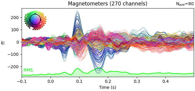
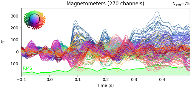
这里我们绘制标准条件和偏差条件的 ERF。在两种条件中都可以看到 P50 和 N100 响应。失匹配负波仅在偏差条件中于 100-200 ms 左右可见。P200 在两种条件中也在约 170 ms 处可见,但在标准条件中强得多。P300 仅在偏差条件中可见(为准备按键而进行决策)。按住鼠标左键并拖动以框选一个区域,即可查看特定时间段的头皮地形图。
evoked_std.plot(window_title="Standard", gfp=True, time_unit="s")
evoked_dev.plot(window_title="Deviant", gfp=True, time_unit="s")
Removing 5 compensators from info because not all compensation channels were picked.
Removing 5 compensators from info because not all compensation channels were picked.
Removing 5 compensators from info because not all compensation channels were picked.
Removing 5 compensators from info because not all compensation channels were picked.
Removing 5 compensators from info because not all compensation channels were picked.
Removing 5 compensators from info because not all compensation channels were picked.
以地形图形式展示激活。
times = np.arange(0.05, 0.301, 0.025)
fig = evoked_std.plot_topomap(times=times)
fig.suptitle("Standard")

fig = evoked_dev.plot_topomap(times=times)
fig.suptitle("Deviant")

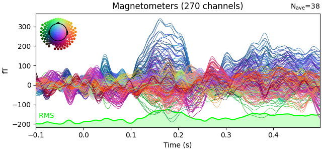
通过观察两种条件之间的差异,我们可以更清楚地看到 MMN 效应。P50 和 N100 不再可见,但 MMN/P200 和 P300 更加突出。
evoked_difference = combine_evoked([evoked_dev, evoked_std], weights=[1, -1])
evoked_difference.plot(window_title="Difference", gfp=True, time_unit="s")
Removing 5 compensators from info because not all compensation channels were picked.
Removing 5 compensators from info because not all compensation channels were picked.
Removing 5 compensators from info because not all compensation channels were picked.
源估计。我们从空房间测量中计算噪声协方差矩阵,并将其用于其他运行。
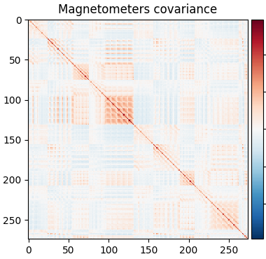
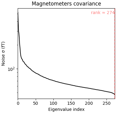
Using up to 150 segments
Number of samples used : 72000
[done]
Removing 5 compensators from info because not all compensation channels were picked.
Computing rank from covariance with rank=None
    Using tolerance 1.7e-14 (2.2e-16 eps * 274 dim * 0.27  max singular value)
    Estimated rank (mag): 274
    MAG: rank 274 computed from 274 data channels with 0 projectors
变换矩阵从文件中读取:
trans_fname = data_path / "MEG" / "bst_auditory" / "bst_auditory-trans.fif"
trans = mne.read_trans(trans_fname)
为节省时间和内存,正向解从文件中读取。若要从头构建正向解,请在脚本开头将 use_precomputed=False。用于构建 BEM 解的头表面从文件中读取。由于数据仅包含 MEG 通道,我们只需内颅骨表面来构建正向解。更多信息:Cortical surface reconstruction with FreeSurfer、mne.setup_source_space()、The Boundary Element Model (BEM)、mne.bem.make_watershed_bem()。
if use_precomputed:
    fwd_fname = data_path / "MEG" / "bst_auditory" / "bst_auditory-meg-oct-6-fwd.fif"
    fwd = mne.read_forward_solution(fwd_fname)
else:
    src = mne.setup_source_space(
        subject, spacing="ico4", subjects_dir=subjects_dir, overwrite=True
    )
    model = mne.make_bem_model(
        subject=subject, ico=4, conductivity=[0.3], subjects_dir=subjects_dir
    )
    bem = mne.make_bem_solution(model)
    fwd = mne.make_forward_solution(evoked_std.info, trans=trans, src=src, bem=bem)

inv = mne.minimum_norm.make_inverse_operator(evoked_std.info, fwd, cov)
snr = 3.0
lambda2 = 1.0 / snr**2
del fwd
Reading forward solution from /home/circleci/mne_data/MNE-brainstorm-data/bst_auditory/MEG/bst_auditory/bst_auditory-meg-oct-6-fwd.fif...
    Reading a source space...
    Computing patch statistics...
    Patch information added...
    Distance information added...
    [done]
    Reading a source space...
    Computing patch statistics...
    Patch information added...
    Distance information added...
    [done]
    2 source spaces read
    Desired named matrix (kind = 3523 (FIFF_MNE_FORWARD_SOLUTION_GRAD)) not available
    Read MEG forward solution (8196 sources, 270 channels, free orientations)
    Source spaces transformed to the forward solution coordinate frame
Converting forward solution to surface orientation
    Average patch normals will be employed in the rotation to the local surface coordinates....
    Converting to surface-based source orientations...
    [done]
info["bads"] and noise_cov["bads"] do not match, excluding bad channels from both
Computing inverse operator with 270 channels.
    270 out of 270 channels remain after picking
Removing 5 compensators from info because not all compensation channels were picked.
Selected 270 channels
Creating the depth weighting matrix...
    270 magnetometer or axial gradiometer channels
    limit = 8033/8196 = 10.015871
    scale = 6.10585e-11 exp = 0.8
Applying loose dipole orientations to surface source spaces: 0.2
Whitening the forward solution.
Removing 5 compensators from info because not all compensation channels were picked.
    Created an SSP operator (subspace dimension = 2)
Computing rank from covariance with rank=None
    Using tolerance 9.8e-15 (2.2e-16 eps * 270 dim * 0.16  max singular value)
    Estimated rank (mag): 268
    MAG: rank 268 computed from 270 data channels with 2 projectors
    Setting small MAG eigenvalues to zero (without PCA)
Creating the source covariance matrix
Adjusting source covariance matrix.
Computing SVD of whitened and weighted lead field matrix.
    largest singular value = 8.09843
    scaling factor to adjust the trace = 3.11765e+19 (nchan = 270 nzero = 2)
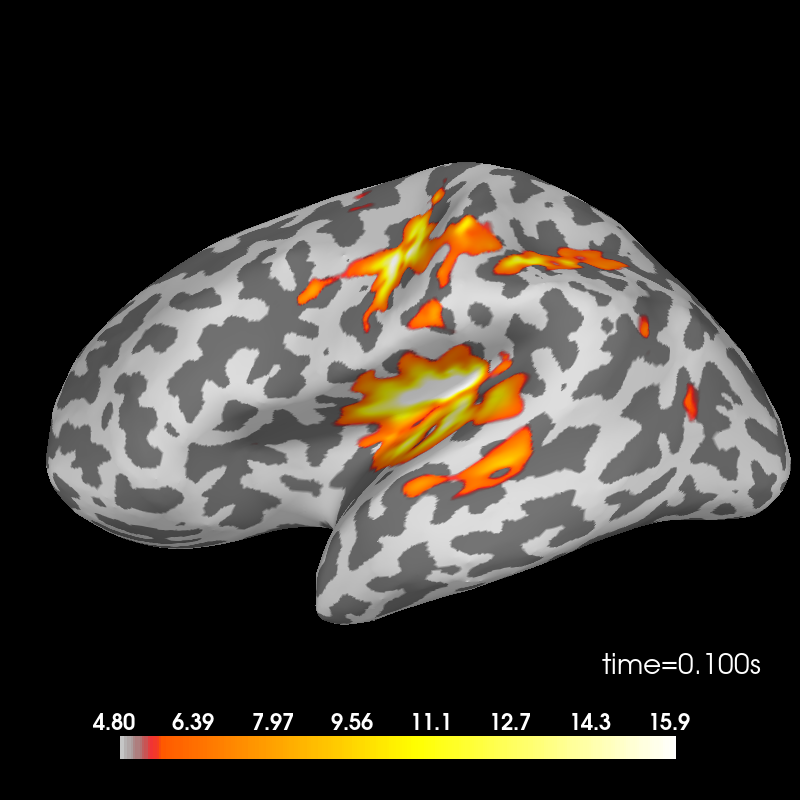
使用 dSPM 方法计算源,并在膨胀的大脑表面上绘制。如需对图像进行交互式控制,请使用关键字参数 time_viewer=True。标准条件。
stc_standard = mne.minimum_norm.apply_inverse(evoked_std, inv, lambda2, "dSPM")
brain = stc_standard.plot(
    subjects_dir=subjects_dir,
    subject=subject,
    surface="inflated",
    time_viewer=False,
    hemi="lh",
    initial_time=0.1,
    time_unit="s",
)
del stc_standard, brain
Removing 5 compensators from info because not all compensation channels were picked.
Preparing the inverse operator for use...
    Scaled noise and source covariance from nave = 1 to nave = 80
    Created the regularized inverter
    Created an SSP operator (subspace dimension = 2)
    Created the whitener using a noise covariance matrix with rank 268 (2 small eigenvalues omitted)
    Computing noise-normalization factors (dSPM)...
[done]
Applying inverse operator to "standard"...
    Picked 270 channels from the data
    Computing inverse...
    Eigenleads need to be weighted ...
    Computing residual...
    Explained  97.0% variance
    Combining the current components...
    dSPM...
[done]
Using control points [ 4.80289065  5.69025561 15.89954825]
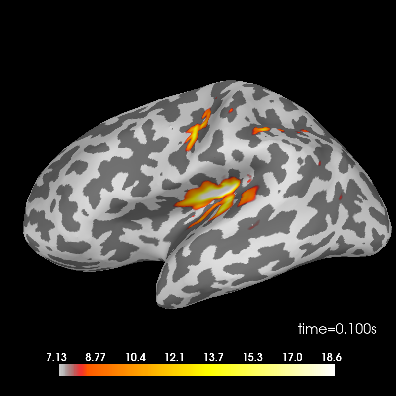
偏差条件。
stc_deviant = mne.minimum_norm.apply_inverse(evoked_dev, inv, lambda2, "dSPM")
brain = stc_deviant.plot(
    subjects_dir=subjects_dir,
    subject=subject,
    surface="inflated",
    time_viewer=False,
    hemi="lh",
    initial_time=0.1,
    time_unit="s",
)
del stc_deviant, brain
Removing 5 compensators from info because not all compensation channels were picked.
Preparing the inverse operator for use...
    Scaled noise and source covariance from nave = 1 to nave = 75
    Created the regularized inverter
    Created an SSP operator (subspace dimension = 2)
    Created the whitener using a noise covariance matrix with rank 268 (2 small eigenvalues omitted)
    Computing noise-normalization factors (dSPM)...
[done]
Applying inverse operator to "deviant"...
    Picked 270 channels from the data
    Computing inverse...
    Eigenleads need to be weighted ...
    Computing residual...
    Explained  98.2% variance
    Combining the current components...
    dSPM...
[done]
Using control points [ 7.12814543  8.29154718 18.6203076 ]
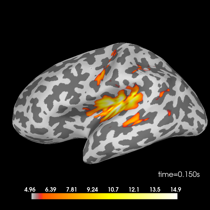
差异。
stc_difference = apply_inverse(evoked_difference, inv, lambda2, "dSPM")
brain = stc_difference.plot(
    subjects_dir=subjects_dir,
    subject=subject,
    surface="inflated",
    time_viewer=False,
    hemi="lh",
    initial_time=0.15,
    time_unit="s",
)
Removing 5 compensators from info because not all compensation channels were picked.
Preparing the inverse operator for use...
    Scaled noise and source covariance from nave = 1 to nave = 38
    Created the regularized inverter
    Created an SSP operator (subspace dimension = 2)
    Created the whitener using a noise covariance matrix with rank 268 (2 small eigenvalues omitted)
    Computing noise-normalization factors (dSPM)...
[done]
Applying inverse operator to "deviant - standard"...
    Picked 270 channels from the data
    Computing inverse...
    Eigenleads need to be weighted ...
    Computing residual...
    Explained  97.2% variance
    Combining the current components...
    dSPM...
[done]
Using control points [ 4.96162575  5.78319301 14.94351171]
参考文献#
脚本总运行时间:(0 分钟 24.957 秒)