非官方中文翻译 本页译自 MNE-Python 官方文档： 查看英文原文 ↗。 文档版权归 MNE Developers 所有（BSD-3-Clause）。

解码（MVPA）

设计理念

MNE 中的解码（又称 MVPA）大体遵循 scikit-learn 包的机器学习 API。每个估计器都实现 fit、transform、fit_transform 以及（可选的）inverse_transform 方法。有关该设计的更多细节，请访问 scikit-learn。关于 MNE 中解码框架的更多理论洞见，请参阅 [1]。

为便于理解，我们用与类名相同、但改为小型大写字母而非驼峰式的名称来表示该类的实例。

首先加载一个简单二分类问题的数据：

import matplotlib.pyplot as plt
import numpy as np
from sklearn.linear_model import LogisticRegression
from sklearn.pipeline import make_pipeline
from sklearn.preprocessing import StandardScaler

import mne
from mne.datasets import sample
from mne.decoding import (
    CSP,
    GeneralizingEstimator,
    LinearModel,
    Scaler,
    SlidingEstimator,
    Vectorizer,
    cross_val_multiscore,
    get_coef,
    get_spatial_filter_from_estimator,
)

data_path = sample.data_path()

subjects_dir = data_path / "subjects"
meg_path = data_path / "MEG" / "sample"
raw_fname = meg_path / "sample_audvis_filt-0-40_raw.fif"
tmin, tmax = -0.200, 0.500
event_id = {"Auditory/Left": 1, "Visual/Left": 3}  # just use two
raw = mne.io.read_raw_fif(raw_fname)
raw.pick(picks=["grad", "stim", "eog"])

# The subsequent decoding analyses only capture evoked responses, so we can
# low-pass the MEG data. Usually a value more like 40 Hz would be used,
# but here low-pass at 20 so we can more heavily decimate, and allow
# the example to run faster. The 2 Hz high-pass helps improve CSP.
raw.load_data().filter(2, 20)
events = mne.find_events(raw, "STI 014")

# Set up bad channels (modify to your needs)
raw.info["bads"] += ["MEG 2443"]  # bads + 2 more

# Read epochs
epochs = mne.Epochs(
    raw,
    events,
    event_id,
    tmin,
    tmax,
    proj=True,
    picks=("grad", "eog"),
    baseline=(None, 0.0),
    preload=True,
    reject=dict(grad=4000e-13, eog=150e-6),
    decim=3,
    verbose="error",
)
epochs.pick(picks="meg", exclude="bads")  # remove stim and EOG
del raw

X = epochs.get_data(copy=False)  # MEG signals: n_epochs, n_meg_channels, n_times
y = epochs.events[:, 2]  # target: auditory left vs visual left

Opening raw data file /home/circleci/mne_data/MNE-sample-data/MEG/sample/sample_audvis_filt-0-40_raw.fif...
    Read a total of 4 projection items:
        PCA-v1 (1 x 102)  idle
        PCA-v2 (1 x 102)  idle
        PCA-v3 (1 x 102)  idle
        Average EEG reference (1 x 60)  idle
    Range : 6450 ... 48149 =     42.956 ...   320.665 secs
Ready.
Reading 0 ... 41699  =      0.000 ...   277.709 secs...
Filtering raw data in 1 contiguous segment
Setting up band-pass filter from 2 - 20 Hz

FIR filter parameters
---------------------
Designing a one-pass, zero-phase, non-causal bandpass filter:
- Windowed time-domain design (firwin) method
- Hamming window with 0.0194 passband ripple and 53 dB stopband attenuation
- Lower passband edge: 2.00
- Lower transition bandwidth: 2.00 Hz (-6 dB cutoff frequency: 1.00 Hz)
- Upper passband edge: 20.00 Hz
- Upper transition bandwidth: 5.00 Hz (-6 dB cutoff frequency: 22.50 Hz)
- Filter length: 249 samples (1.658 s)

Finding events on: STI 014
319 events found on stim channel STI 014
Event IDs: [ 1  2  3  4  5 32]

变换类

Scaler

mne.decoding.Scaler 会基于通道尺度对数据进行标准化。在最简单的模式 scalings=None 或 scalings=dict(...) 下，每种数据通道类型（如 mag、grad、eeg）分别处理，并用一个常数进行缩放。例如 mne.compute_covariance() 就采用这种方式来标准化通道尺度。

若 scalings='mean' 或 scalings='median'，则每个通道使用经验性度量进行缩放。在 fit（训练）期间，每个通道分别按所有分段和时间点上的均值与标准差，或中位数与四分位距进行独立缩放。调用 transform() 方法时，会按通道对所有时间点和分段进行缩放，以变换数据（训练集或测试集）。若要在一次调用中同时完成拟合与变换，可使用 fit_transform() 方法。要逆转变换，可使用 inverse_transform()。使用 scalings='median' 需要 scikit-learn 0.17 或更高版本。

注意

使用该类与直接使用 scikit-learn 提供的 sklearn.preprocessing.StandardScaler 或 sklearn.preprocessing.RobustScaler 不同。后者会对每个分类特征（例如每个通道的每个时间点）进行缩放，其均值和标准差是在分段维度上计算的；而 mne.decoding.Scaler 则使用该通道所有时间点和全部分段上计算得到的均值和标准差来缩放每个通道。

Vectorizer

scikit-learn API 通过 sklearn.pipeline.Pipeline 提供了将变换器与估计器串联起来的功能。我们可以构建解码流水线，并执行交叉验证和网格搜索。然而，scikit-learn 的变换器和估计器通常期望 2D 数据（n_samples * n_features），而 MNE 的变换器通常输出维度更高的数据（例如 n_samples * n_channels * n_frequencies * n_times）。因此需要在 MNE 与 scikit-learn 步骤之间应用 Vectorizer，如下所示：

# Uses all MEG sensors and time points as separate classification
# features, so the resulting filters used are spatio-temporal
clf = make_pipeline(
    Scaler(epochs.info),
    Vectorizer(),
    # liblinear is faster than lbfgs
    LogisticRegression(solver="liblinear", random_state=31),
)

scores = cross_val_multiscore(clf, X, y, cv=5, n_jobs=None)

# Mean scores across cross-validation splits
score = np.mean(scores, axis=0)
print(f"Spatio-temporal: {100 * score:0.1f}%")

Spatio-temporal: 99.2%

PSDEstimator

mne.decoding.PSDEstimator 使用多锥度（multitaper）方法计算功率谱密度（PSD）。它接收 3D 数组作为输入，将其转换为 2D 后计算 PSD。

FilterEstimator

mne.decoding.FilterEstimator 对 3D 的分段数据进行滤波。

空间滤波器

与时域滤波器类似，空间滤波器提供权重，沿传感器维度修改数据。由于简单且能够区分空间上分离的神经活动，空间滤波器在 BCI 领域很受欢迎。

共空间模式

mne.decoding.CSP 是一种基于两类记录分析多通道数据的技术 [2]（另见 https://en.wikipedia.org/wiki/Common_spatial_pattern）。

设 \(X \in R^{C\times T}\) 为包含 \(C\) 个通道和 \(T\) 个时间点的数据段。单个时间点的数据记为 \(x(t)\)，因此 \(X=[x(t), x(t+1), ..., x(t+T-1)]\)。共空间模式（CSP）寻找一种分解，通过以下变换将原始传感器空间中的信号投影到 CSP 空间：

(1)\[x_{CSP}(t) = W^{T}x(t)\]

其中 \(W \in R^{C\times C}\) 的每一列是一个空间滤波器，\(x_{CSP}\) 的每一行是一个 CSP 成分。矩阵 \(W\) 在其他语境中也称为解混矩阵（de-mixing matrix）。设 \(\Sigma^{+} \in R^{C\times C}\) 和 \(\Sigma^{-} \in R^{C\times C}\) 为两个条件下协方差矩阵的估计，则 CSP 分析通过对两个协方差矩阵进行同时对角化给出：

(2)\[W^{T}\Sigma^{+}W = \lambda^{+}\]

(3)\[W^{T}\Sigma^{-}W = \lambda^{-}\]

其中 \(\lambda^{C}\) 是一个对角矩阵，其元素为以下广义特征值问题的特征值：

(4)\[\Sigma^{+}w = \lambda \Sigma^{-}w\]

对角矩阵中的大元素对应一个空间滤波器，它在某一类别中产生高方差，而在另一类别中产生低方差。因此，该滤波器有助于区分这两个类别。

示例

• 使用共空间模式（CSP）从 EEG 数据解码运动想象

• 使用共空间模式（CSP）在时频空间中进行解码

注意

Kaggle 上 Grasp-and-lift EEG 竞赛的获胜方案使用了 MNE 中的 CSP 实现，并被作为“当周脚本”（script of the week）展示。

可以对这些数据使用 CSP，如下所示：

csp = CSP(n_components=3, norm_trace=False)
clf_csp = make_pipeline(
    csp, LinearModel(LogisticRegression(solver="liblinear", random_state=37))
)
scores = cross_val_multiscore(clf_csp, X, y, cv=5, n_jobs=None)
print(f"CSP: {100 * scores.mean():0.1f}%")

Computing rank from data with rank=None
    Using tolerance 6e-11 (2.2e-16 eps * 203 dim * 1.3e+03  max singular value)
    Estimated rank (data): 203
    data: rank 203 computed from 203 data channels with 0 projectors
Reducing data rank from 203 -> 203
Estimating class=1 covariance using EMPIRICAL
Done.
Estimating class=3 covariance using EMPIRICAL
Done.
Computing rank from data with rank=None
    Using tolerance 6e-11 (2.2e-16 eps * 203 dim * 1.3e+03  max singular value)
    Estimated rank (data): 203
    data: rank 203 computed from 203 data channels with 0 projectors
Reducing data rank from 203 -> 203
Estimating class=1 covariance using EMPIRICAL
Done.
Estimating class=3 covariance using EMPIRICAL
Done.
Computing rank from data with rank=None
    Using tolerance 6e-11 (2.2e-16 eps * 203 dim * 1.3e+03  max singular value)
    Estimated rank (data): 203
    data: rank 203 computed from 203 data channels with 0 projectors
Reducing data rank from 203 -> 203
Estimating class=1 covariance using EMPIRICAL
Done.
Estimating class=3 covariance using EMPIRICAL
Done.
Computing rank from data with rank=None
    Using tolerance 5.8e-11 (2.2e-16 eps * 203 dim * 1.3e+03  max singular value)
    Estimated rank (data): 203
    data: rank 203 computed from 203 data channels with 0 projectors
Reducing data rank from 203 -> 203
Estimating class=1 covariance using EMPIRICAL
Done.
Estimating class=3 covariance using EMPIRICAL
Done.
Computing rank from data with rank=None
    Using tolerance 5.9e-11 (2.2e-16 eps * 203 dim * 1.3e+03  max singular value)
    Estimated rank (data): 203
    data: rank 203 computed from 203 data channels with 0 projectors
Reducing data rank from 203 -> 203
Estimating class=1 covariance using EMPIRICAL
Done.
Estimating class=3 covariance using EMPIRICAL
Done.
CSP: 89.4%

源功率共调制（SPoC）

源功率共调制（Source Power Comodulation，mne.decoding.SPoC）[3] 找出与连续目标最大相关的正交空间滤波器组合。

SPoC 可视为 CSP 的扩展，其中目标由连续变量而非离散变量驱动。典型应用包括使用 EMG 功率提取运动模式，或使用声音包络提取听觉模式。

示例

• 使用 SPoC 进行连续目标解码

xDAWN

mne.preprocessing.Xdawn 是一种空间滤波方法，旨在提高 ERP 响应的信号与信号加噪声比（SSNR）[4]。Xdawn 最初针对 P300 诱发电位设计，通过增强目标响应相对于非目标响应的强度来工作。MNE-Python 中的实现可推广到任意类型的 ERP。

示例

• XDAWN 去噪

• 基于 EEG 数据的 XDAWN 解码

效应匹配空间滤波

mne.decoding.EMS 的结果是每个时间点上的一个空间滤波器及对应的时间进程 [5]。直观地说，该结果给出了每个时间点的滤波器与该时间点数据向量（传感器）之间的相似性。

示例

• 计算效应匹配空间滤波（EMS）

模式与滤波器

在解释 CSP 成分（或一般的空间滤波器）时，思考 \(x(t)\) 如何由不同的 CSP 成分 \(x_{CSP}(t)\) 构成往往更直观。换言之，我们可以将公式 (1) 改写如下：

(5)\[x(t) = (W^{-1})^{T}x_{CSP}(t)\]

矩阵 \((W^{-1})^T\) 的各列称为空间模式（spatial patterns），也称为混合矩阵（mixing matrix）。示例“在传感器数据上使用线性分类器并绘制模式与滤波器”讨论了模式与滤波器之间的区别。

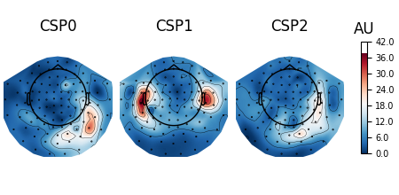
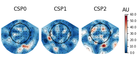
可以对每个空间滤波器（包括 CSP、XdawnTransformer、SSD 和 SPoC）绘制这些内容：

# Fit CSP on full data, plot eigenvalues sorted based on mutual information,
# and plot patterns and filters for the three components largest components.
csp.fit(X, y)
spf = get_spatial_filter_from_estimator(csp, info=epochs.info)
spf.plot_scree()
spf.plot_patterns(components=[0, 1, 2])
spf.plot_filters(components=[0, 1, 2], scalings=1e-9)

• 
• 
• 

Computing rank from data with rank=None
    Using tolerance 6.6e-11 (2.2e-16 eps * 203 dim * 1.5e+03  max singular value)
    Estimated rank (data): 203
    data: rank 203 computed from 203 data channels with 0 projectors
Reducing data rank from 203 -> 203
Estimating class=1 covariance using EMPIRICAL
Done.
Estimating class=3 covariance using EMPIRICAL
Done.

沿时间解码

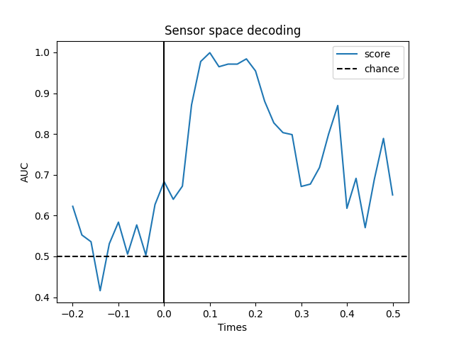
该策略在每个时间点上拟合一个多变量预测模型，并在新分段上评估模型在同一时间点的表现。mne.decoding.SlidingEstimator 接收一对特征 \(X\) 和目标 \(y\) 作为输入，其中 \(X\) 具有两个以上的维度。对于随时间解码，数据 \(X\) 是形状为 n_epochs × n_channels × n_times 的分段数据。由于 \(X\) 的最后一维是时间，因此会在每个时间点上拟合一个估计器。

这种方法类似于 fMRI 中基于 SlidingEstimator 的方法；在这里，我们关注的是何时能够区分实验条件，从而确定感兴趣效应发生的时间。

当使用线性模型作为估计器时，这种方法实际上就是为每个时间点估计一个判别性空间滤波器。

时间解码

我们将使用逻辑回归（Logistic Regression）作为机器学习模型进行二分类。

# We will train the classifier on all left visual vs auditory trials on MEG

clf = make_pipeline(
    StandardScaler(), LogisticRegression(solver="liblinear", random_state=41)
)

time_decod = SlidingEstimator(clf, n_jobs=None, scoring="roc_auc", verbose=True)
# here we use cv=3 just for speed
scores = cross_val_multiscore(time_decod, X, y, cv=3, n_jobs=None)

# Mean scores across cross-validation splits
scores = np.mean(scores, axis=0)

# Plot
fig, ax = plt.subplots()
ax.plot(epochs.times, scores, label="score")
ax.axhline(0.5, color="k", linestyle="--", label="chance")
ax.set_xlabel("Times")
ax.set_ylabel("AUC")  # Area Under the Curve
ax.legend()
ax.axvline(0.0, color="k", linestyle="-")
ax.set_title("Sensor space decoding")

  0%|          | Fitting SlidingEstimator : 0/36 [00:00<?,       ?it/s]
 31%|███       | Fitting SlidingEstimator : 11/36 [00:00<00:00,  326.50it/s]
 69%|██████▉   | Fitting SlidingEstimator : 25/36 [00:00<00:00,  372.86it/s]
100%|██████████| Fitting SlidingEstimator : 36/36 [00:00<00:00,  388.98it/s]
100%|██████████| Fitting SlidingEstimator : 36/36 [00:00<00:00,  386.65it/s]

  0%|          | Fitting SlidingEstimator : 0/36 [00:00<?,       ?it/s]
 33%|███▎      | Fitting SlidingEstimator : 12/36 [00:00<00:00,  355.28it/s]
 75%|███████▌  | Fitting SlidingEstimator : 27/36 [00:00<00:00,  400.37it/s]
100%|██████████| Fitting SlidingEstimator : 36/36 [00:00<00:00,  398.62it/s]
100%|██████████| Fitting SlidingEstimator : 36/36 [00:00<00:00,  397.33it/s]

  0%|          | Fitting SlidingEstimator : 0/36 [00:00<?,       ?it/s]
 33%|███▎      | Fitting SlidingEstimator : 12/36 [00:00<00:00,  353.73it/s]
 72%|███████▏  | Fitting SlidingEstimator : 26/36 [00:00<00:00,  386.02it/s]
100%|██████████| Fitting SlidingEstimator : 36/36 [00:00<00:00,  398.60it/s]
100%|██████████| Fitting SlidingEstimator : 36/36 [00:00<00:00,  396.62it/s]

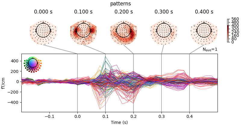
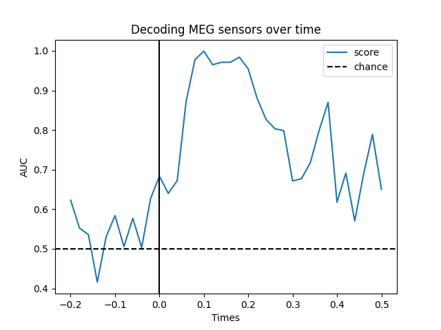
如果显式使用 LinearModel，则可以获取空间滤波器和空间模式：

clf = make_pipeline(
    StandardScaler(),
    LinearModel(LogisticRegression(solver="liblinear", random_state=43)),
)
time_decod = SlidingEstimator(clf, n_jobs=None, scoring="roc_auc", verbose=True)
time_decod.fit(X, y)

coef = get_coef(time_decod, "patterns_", inverse_transform=True)
evoked_time_gen = mne.EvokedArray(coef, epochs.info, tmin=epochs.times[0])
joint_kwargs = dict(ts_args=dict(time_unit="s"), topomap_args=dict(time_unit="s"))
evoked_time_gen.plot_joint(
    times=np.arange(0.0, 0.500, 0.100), title="patterns", **joint_kwargs
)

  0%|          | Fitting SlidingEstimator : 0/36 [00:00<?,       ?it/s]
 19%|█▉        | Fitting SlidingEstimator : 7/36 [00:00<00:00,  207.96it/s]
 44%|████▍     | Fitting SlidingEstimator : 16/36 [00:00<00:00,  235.63it/s]
 69%|██████▉   | Fitting SlidingEstimator : 25/36 [00:00<00:00,  247.11it/s]
 92%|█████████▏| Fitting SlidingEstimator : 33/36 [00:00<00:00,  244.84it/s]
100%|██████████| Fitting SlidingEstimator : 36/36 [00:00<00:00,  251.34it/s]
No projector specified for this dataset. Please consider the method self.add_proj.

时间泛化

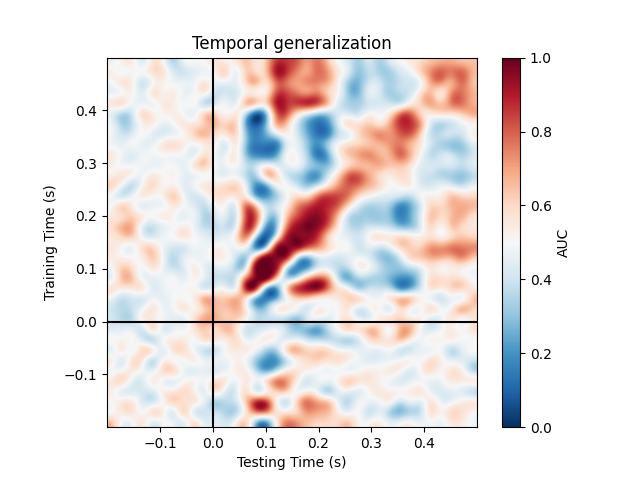
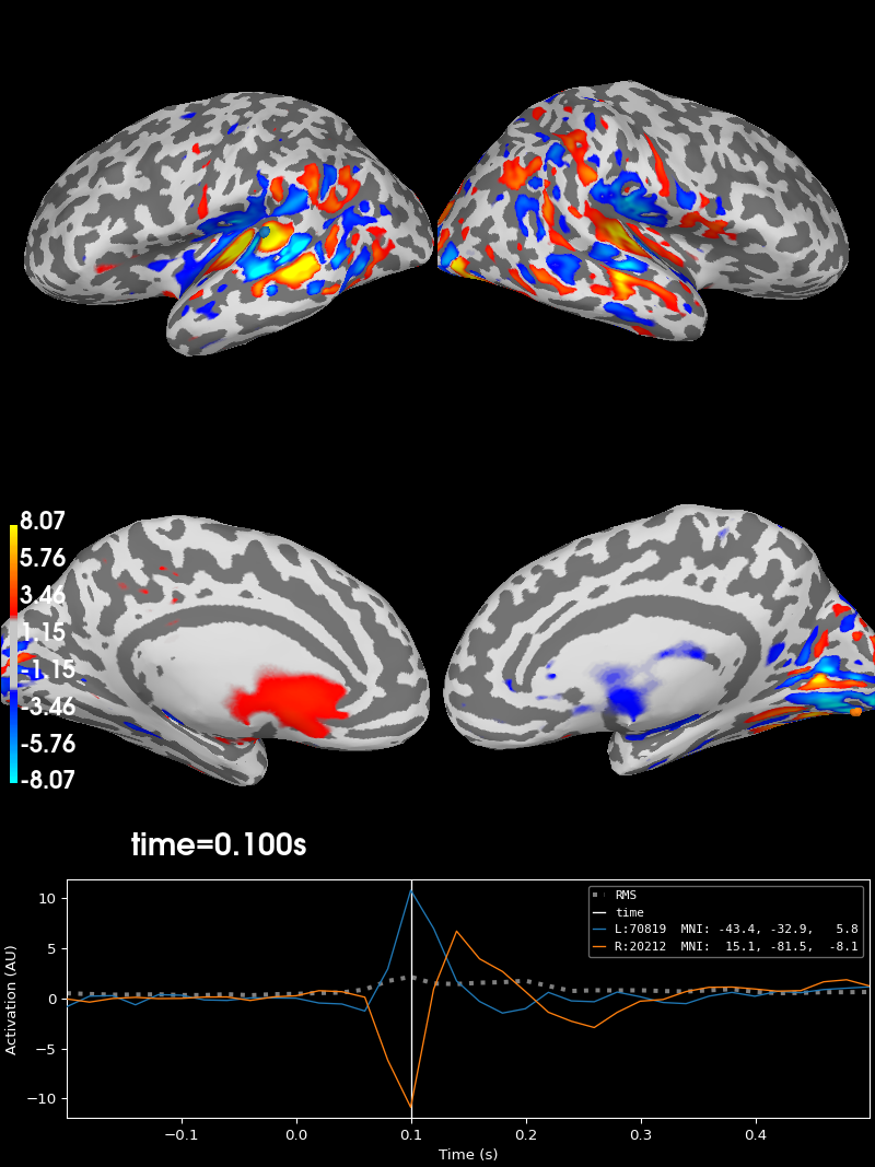
时间泛化是沿时间解码方法的扩展。它评估在某一特定时间点估计的模型能否准确预测任何其他时间点。这类似于将训练好的模型迁移到一个不同的学习问题，其中不同的问题对应于解码在不同时间点记录的大脑活动模式。

用于时间泛化的对象是 mne.decoding.GeneralizingEstimator。它期望输入 \(X\) 和 \(y\)（与 SlidingEstimator 类似），但会为所有时间点生成每个模型的预测。GeneralizingEstimator 类是通用的，会将最后一维视为用于泛化测试的维度。为方便起见，这里我们将其称为不同的任务。如果 \(X\) 对应分段数据，则最后一维是时间。

这里运行的是 [6] 中使用的分析，[7] 对其做了进一步详述：

# define the Temporal generalization object
time_gen = GeneralizingEstimator(clf, n_jobs=None, scoring="roc_auc", verbose=True)

# again, cv=3 just for speed
scores = cross_val_multiscore(time_gen, X, y, cv=3, n_jobs=None)

# Mean scores across cross-validation splits
scores = np.mean(scores, axis=0)

# Plot the diagonal (it's exactly the same as the time-by-time decoding above)
fig, ax = plt.subplots()
ax.plot(epochs.times, np.diag(scores), label="score")
ax.axhline(0.5, color="k", linestyle="--", label="chance")
ax.set_xlabel("Times")
ax.set_ylabel("AUC")
ax.legend()
ax.axvline(0.0, color="k", linestyle="-")
ax.set_title("Decoding MEG sensors over time")

  0%|          | Fitting GeneralizingEstimator : 0/36 [00:00<?,       ?it/s]
 31%|███       | Fitting GeneralizingEstimator : 11/36 [00:00<00:00,  319.03it/s]
 67%|██████▋   | Fitting GeneralizingEstimator : 24/36 [00:00<00:00,  353.50it/s]
 97%|█████████▋| Fitting GeneralizingEstimator : 35/36 [00:00<00:00,  344.56it/s]
100%|██████████| Fitting GeneralizingEstimator : 36/36 [00:00<00:00,  351.46it/s]

  0%|          | Scoring GeneralizingEstimator : 0/1296 [00:00<?,       ?it/s]
  3%|▎         | Scoring GeneralizingEstimator : 36/1296 [00:00<00:00, 1580.72it/s]
  3%|▎         | Scoring GeneralizingEstimator : 36/1296 [00:00<00:00, 1570.15it/s]

  0%|          | Fitting GeneralizingEstimator : 0/36 [00:00<?,       ?it/s]
 31%|███       | Fitting GeneralizingEstimator : 11/36 [00:00<00:00,  327.20it/s]
 64%|██████▍   | Fitting GeneralizingEstimator : 23/36 [00:00<00:00,  339.96it/s]
 97%|█████████▋| Fitting GeneralizingEstimator : 35/36 [00:00<00:00,  345.23it/s]
100%|██████████| Fitting GeneralizingEstimator : 36/36 [00:00<00:00,  345.33it/s]

  0%|          | Scoring GeneralizingEstimator : 0/1296 [00:00<?,       ?it/s]
  3%|▎         | Scoring GeneralizingEstimator : 36/1296 [00:00<00:00, 1561.16it/s]
  3%|▎         | Scoring GeneralizingEstimator : 36/1296 [00:00<00:00, 1550.73it/s]

  0%|          | Fitting GeneralizingEstimator : 0/36 [00:00<?,       ?it/s]
 31%|███       | Fitting GeneralizingEstimator : 11/36 [00:00<00:00,  318.87it/s]
 64%|██████▍   | Fitting GeneralizingEstimator : 23/36 [00:00<00:00,  338.44it/s]
 97%|█████████▋| Fitting GeneralizingEstimator : 35/36 [00:00<00:00,  342.44it/s]
100%|██████████| Fitting GeneralizingEstimator : 36/36 [00:00<00:00,  347.51it/s]

  0%|          | Scoring GeneralizingEstimator : 0/1296 [00:00<?,       ?it/s]
  3%|▎         | Scoring GeneralizingEstimator : 36/1296 [00:00<00:00, 1555.22it/s]
  3%|▎         | Scoring GeneralizingEstimator : 36/1296 [00:00<00:00, 1544.75it/s]

绘制完整的（泛化）矩阵：

fig, ax = plt.subplots(1, 1)
im = ax.imshow(
    scores,
    interpolation="lanczos",
    origin="lower",
    cmap="RdBu_r",
    extent=epochs.times[[0, -1, 0, -1]],
    vmin=0.0,
    vmax=1.0,
)
ax.set_xlabel("Testing Time (s)")
ax.set_ylabel("Training Time (s)")
ax.set_title("时间泛化")
ax.axvline(0, color="k")
ax.axhline(0, color="k")
cbar = plt.colorbar(im, ax=ax)
cbar.set_label("AUC")

将传感器空间模式投影到源空间

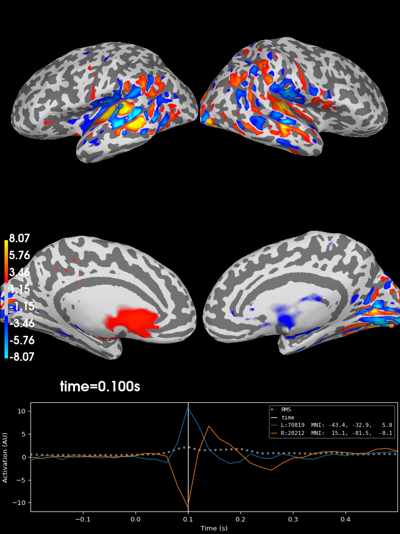
如果对数据使用线性分类器（或回归器），也可以将这些模式投影到源空间。例如，使用前面的 evoked_time_gen：

cov = mne.compute_covariance(epochs, tmax=0.0)
del epochs
fwd = mne.read_forward_solution(meg_path / "sample_audvis-meg-eeg-oct-6-fwd.fif")
inv = mne.minimum_norm.make_inverse_operator(evoked_time_gen.info, fwd, cov, loose=0.0)
stc = mne.minimum_norm.apply_inverse(evoked_time_gen, inv, 1.0 / 9.0, "dSPM")
del fwd, inv

Reducing data rank from 203 -> 203
Estimating covariance using EMPIRICAL
Done.
Number of samples used : 1353
[done]
Reading forward solution from /home/circleci/mne_data/MNE-sample-data/MEG/sample/sample_audvis-meg-eeg-oct-6-fwd.fif...
    Reading a source space...
    Computing patch statistics...
    Patch information added...
    Distance information added...
    [done]
    Reading a source space...
    Computing patch statistics...
    Patch information added...
    Distance information added...
    [done]
    2 source spaces read
    Desired named matrix (kind = 3523 (FIFF_MNE_FORWARD_SOLUTION_GRAD)) not available
    Read MEG forward solution (7498 sources, 306 channels, free orientations)
    Desired named matrix (kind = 3523 (FIFF_MNE_FORWARD_SOLUTION_GRAD)) not available
    Read EEG forward solution (7498 sources, 60 channels, free orientations)
    Forward solutions combined: MEG, EEG
    Source spaces transformed to the forward solution coordinate frame
Computing inverse operator with 203 channels.
    203 out of 366 channels remain after picking
Selected 203 channels
Creating the depth weighting matrix...
    203 planar channels
    limit = 7262/7498 = 10.020866
    scale = 2.58122e-08 exp = 0.8
    Picked elements from a free-orientation depth-weighting prior into the fixed-orientation one
    Average patch normals will be employed in the rotation to the local surface coordinates....
    Converting to surface-based source orientations...
    [done]
Whitening the forward solution.
Computing rank from covariance with rank=None
    Using tolerance 1.6e-13 (2.2e-16 eps * 203 dim * 3.6  max singular value)
    Estimated rank (grad): 203
    GRAD: rank 203 computed from 203 data channels with 0 projectors
    Setting small GRAD eigenvalues to zero (without PCA)
Creating the source covariance matrix
Adjusting source covariance matrix.
Computing SVD of whitened and weighted lead field matrix.
    largest singular value = 3.91709
    scaling factor to adjust the trace = 6.26373e+18 (nchan = 203 nzero = 0)
Preparing the inverse operator for use...
    Scaled noise and source covariance from nave = 1 to nave = 1
    Created the regularized inverter
    The projection vectors do not apply to these channels.
    Created the whitener using a noise covariance matrix with rank 203 (0 small eigenvalues omitted)
    Computing noise-normalization factors (dSPM)...
[done]
Applying inverse operator to ""...
    Picked 203 channels from the data
    Computing inverse...
    Eigenleads need to be weighted ...
    Computing residual...
    Explained  76.4% variance
    dSPM...
[done]

可以使用 stc.plot 进行可视化：

brain = stc.plot(
    hemi="split", views=("lat", "med"), initial_time=0.1, subjects_dir=subjects_dir
)

Using control points [1.98776221 2.41838256 8.06628583]

源空间解码

源空间解码同样可行，但由于特征数量可能远多于传感器空间，因此可以使用 ANOVA f 检验（或其他指标）进行单变量特征选择，以降低特征维度。与传感器空间相比，源空间中的解码结果可能更易于解释。

示例

• 解码源空间数据

练习

• 探索 MNE 的其他数据集（例如使用 SPM 的 Face 数据集预测 Face 与 Scrambled）

参考文献

[1]

Jean-Rémi King, Laura Gwilliams, Chris Holdgraf, Jona Sassenhagen, Alexandre Barachant, Denis Engemann, Eric Larson, and Alexandre Gramfort. Encoding and decoding neuronal dynamics: methodological framework to uncover the algorithms of cognition. hal-01848442, 2018. URL: https://hal.archives-ouvertes.fr/hal-01848442.

[2]

Zoltan J. Koles. The quantitative extraction and topographic mapping of the abnormal components in the clinical EEG. Electroencephalography and Clinical Neurophysiology, 79(6):440–447, 1991. doi:10.1016/0013-4694(91)90163-X.

[3]

Sven Dähne, Frank C. Meinecke, Stefan Haufe, Johannes Höhne, Michael Tangermann, Klaus-Robert Müller, and Vadim V. Nikulin. SPoC: a novel framework for relating the amplitude of neuronal oscillations to behaviorally relevant parameters. NeuroImage, 86:111–122, 2014. doi:10.1016/j.neuroimage.2013.07.079.

[4]

Bertrand Rivet, Antoine Souloumiac, Virginie Attina, and Guillaume Gibert. xDAWN algorithm to enhance evoked potentials: application to brain–computer interface. IEEE Transactions on Biomedical Engineering, 56(8):2035–2043, 2009. doi:10.1109/TBME.2009.2012869.

[5]

Aaron Schurger, Sebastien Marti, and Stanislas Dehaene. Reducing multi-sensor data to a single time course that reveals experimental effects. BMC Neuroscience, 2013. doi:10.1186/1471-2202-14-122.

[6]

Jean-Rémi King, Alexandre Gramfort, Aaron Schurger, Lionel Naccache, and Stanislas Dehaene. Two distinct dynamic modes subtend the detection of unexpected sounds. PLoS ONE, 9(1):e85791, 2014. doi:10.1371/journal.pone.0085791.

[7]

Jean-Rémi King and Stanislas Dehaene. Characterizing the dynamics of mental representations: the temporal generalization method. Trends in Cognitive Sciences, 18(4):203–210, 2014. doi:10.1016/j.tics.2014.01.002.