
说明
转到末尾下载完整示例代码。
使用 DICS 进行功率映射#
在本教程中,我们将仿真来自皮层上两个位置的两个信号。这些信号为正弦波,因此我们将关注振荡活动(而非诱发活动)。
我们将使用动态相干源成像(dynamic imaging of coherent sources,DICS)[ 1 ] 来绘制沿皮层的频谱功率分布。让我们看看能否找到这两个仿真源。
# Author: Marijn van Vliet <w.m.vanvliet@gmail.com>
#
# License: BSD-3-Clause
# Copyright the MNE-Python contributors.
准备工作#
我们首先导入运行本教程所需的软件包,并为将要使用的各种文件定义一个文件名列表。
import numpy as np
from matplotlib import pyplot as plt
from scipy.signal import coherence, unit_impulse, welch

import mne
from mne.beamformer import apply_dics_csd, make_dics
from mne.datasets import sample
from mne.minimum_norm import apply_inverse, make_inverse_operator
from mne.simulation import add_noise, simulate_raw
from mne.time_frequency import csd_morlet

# We use the MEG and MRI setup from the MNE-sample dataset
data_path = sample.data_path(download=False)
subjects_dir = data_path / "subjects"

# Filenames for various files we'll be using
meg_path = data_path / "MEG" / "sample"
raw_fname = meg_path / "sample_audvis_raw.fif"
fwd_fname = meg_path / "sample_audvis-meg-eeg-oct-6-fwd.fif"
cov_fname = meg_path / "sample_audvis-cov.fif"
fwd = mne.read_forward_solution(fwd_fname)

# Seed for the random number generator
rand = np.random.default_rng(42)
Reading forward solution from /home/circleci/mne_data/MNE-sample-data/MEG/sample/sample_audvis-meg-eeg-oct-6-fwd.fif...
    Reading a source space...
    Computing patch statistics...
    Patch information added...
    Distance information added...
    [done]
    Reading a source space...
    Computing patch statistics...
    Patch information added...
    Distance information added...
    [done]
    2 source spaces read
    Desired named matrix (kind = 3523 (FIFF_MNE_FORWARD_SOLUTION_GRAD)) not available
    Read MEG forward solution (7498 sources, 306 channels, free orientations)
    Desired named matrix (kind = 3523 (FIFF_MNE_FORWARD_SOLUTION_GRAD)) not available
    Read EEG forward solution (7498 sources, 60 channels, free orientations)
    Forward solutions combined: MEG, EEG
    Source spaces transformed to the forward solution coordinate frame
数据仿真#
下面的函数生成一个包含振荡器的时间序列,其频率会随时间略有波动,但始终保持在 10 Hz 附近。我们将用该函数生成两个信号。
sfreq = 50.0  # Sampling frequency of the generated signal
n_samp = int(round(10.0 * sfreq))
times = np.arange(n_samp) / sfreq  # 10 seconds of signal
n_times = len(times)


def coh_signal_gen():
    """Generate an oscillating signal.

    Returns
    -------
    signal : ndarray
        The generated signal.
    """
    t_rand = 0.001  # Variation in the instantaneous frequency of the signal
    std = 0.1  # Std-dev of the random fluctuations added to the signal
    base_freq = 10.0  # Base frequency of the oscillators in Hertz
    n_times = len(times)

    # Generate an oscillator with varying frequency and phase lag.
    signal = np.sin(
        2.0
        * np.pi
        * (
            base_freq * np.arange(n_times) / sfreq
            + np.cumsum(rand.normal(scale=t_rand, size=n_times))
        )
    )

    # Add some random fluctuations to the signal.
    signal += rand.normal(scale=std, size=n_times)

    # Scale the signal to be in the right order of magnitude (~100 nAm)
    # for MEG data.
    signal *= 100e-9

    return signal
让我们仿真两个时间序列,并绘制一些关于它们的基本信息。
signal1 = coh_signal_gen()
signal2 = coh_signal_gen()

fig, axes = plt.subplots(2, 2, figsize=(8, 4), layout="constrained")

# Plot the timeseries
ax = axes[0][0]
ax.plot(times, 1e9 * signal1, lw=0.5)
ax.set(
    xlabel="Time (s)", xlim=times[[0, -1]], ylabel="Amplitude (Am)", title="Signal 1"
)
ax = axes[0][1]
ax.plot(times, 1e9 * signal2, lw=0.5)
ax.set(xlabel="Time (s)", xlim=times[[0, -1]], title="Signal 2")

# Power spectrum of the first timeseries
f, p = welch(signal1, fs=sfreq, nperseg=128, nfft=256)
ax = axes[1][0]
# Only plot the first 100 frequencies
ax.plot(f[:100], 20 * np.log10(p[:100]), lw=1.0)
ax.set(
    xlabel="Frequency (Hz)",
    xlim=f[[0, 99]],
    ylabel="Power (dB)",
    title="Power spectrum of signal 1",
)

# Compute the coherence between the two timeseries
f, coh = coherence(signal1, signal2, fs=sfreq, nperseg=100, noverlap=64)
ax = axes[1][1]
ax.plot(f[:50], coh[:50], lw=1.0)
ax.set(
    xlabel="Frequency (Hz)",
    xlim=f[[0, 49]],
    ylabel="Coherence",
    title="Coherence between the timeseries",
)
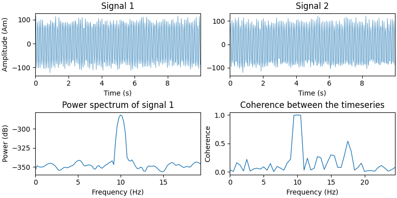
现在我们把信号放到皮层上的两个位置。我们构造一个 mne.SourceEstimate 对象来存储它们。
该时间序列将包含信号活跃的片段和不活跃的片段。本教程中使用的技术依赖于能够对比包含感兴趣信号的数据与不包含信号(即仅含噪声)的数据。
# The locations on the cortex where the signal will originate from. These
# locations are indicated as vertex numbers.
vertices = [[146374], [33830]]

# Construct SourceEstimates that describe the signals at the cortical level.
data = np.vstack((signal1, signal2))
stc_signal = mne.SourceEstimate(
    data, vertices, tmin=0, tstep=1.0 / sfreq, subject="sample"
)
stc_noise = stc_signal * 0.0
在仿真传感器级数据之前,我们先定义一个信噪比。建议您尝试调整该参数,观察噪声对结果的影响。
snr = 1.0 # Signal-to-noise ratio. Decrease to add more noise.
现在我们让信号通过正向模型,以获得仿真的传感器数据。为节省计算时间,我们只仿真梯度计数据。您也可以尝试仿真其他类型的传感器。
我们基于样本数据集的基线噪声协方差矩阵加入一些噪声,并按所需的信噪比进行缩放。
# Read the info from the sample dataset. This defines the location of the
# sensors and such.
info = mne.io.read_raw(raw_fname).crop(0, 1).resample(50).info

# Only use gradiometers
picks = mne.pick_types(info, meg="grad", stim=True, exclude=())
mne.pick_info(info, picks, copy=False)  # modifies info in-place

# Define a covariance matrix for the simulated noise. In this tutorial, we use
# a simple diagonal matrix.
cov = mne.cov.make_ad_hoc_cov(info)
cov["data"] *= (20.0 / snr) ** 2  # Scale the noise to achieve the desired SNR

# Simulate the raw data, with a lowpass filter on the noise
stcs = [
    (stc_signal, unit_impulse(n_samp, dtype=int) * 1),
    (stc_noise, unit_impulse(n_samp, dtype=int) * 2),
]  # stacked in time
duration = (len(stc_signal.times) * 2) / sfreq
raw = simulate_raw(info, stcs, forward=fwd)
add_noise(raw, cov, iir_filter=[4, -4, 0.8], rng=rand)
Opening raw data file /home/circleci/mne_data/MNE-sample-data/MEG/sample/sample_audvis_raw.fif...
    Read a total of 3 projection items:
        PCA-v1 (1 x 10²)  idle
        PCA-v2 (1 x 10²)  idle
        PCA-v3 (1 x 10²)  idle
    Range : 25800 ... 192599 =     42.956 ...   320.670 secs
Ready.
Finding events on: STI 014
Finding events on: STI 014
Setting up raw simulation: 1 position, "cos2" interpolation
Event information stored on channel:              STI 014
    Interval 0.000–10.000 s
Setting up forward solutions
Computing gain matrix for transform #1/1
    Interval 0.000–10.000 s
    2 STC iterations provided
[done]
Adding noise to 204/213 channels (204 channels in cov)
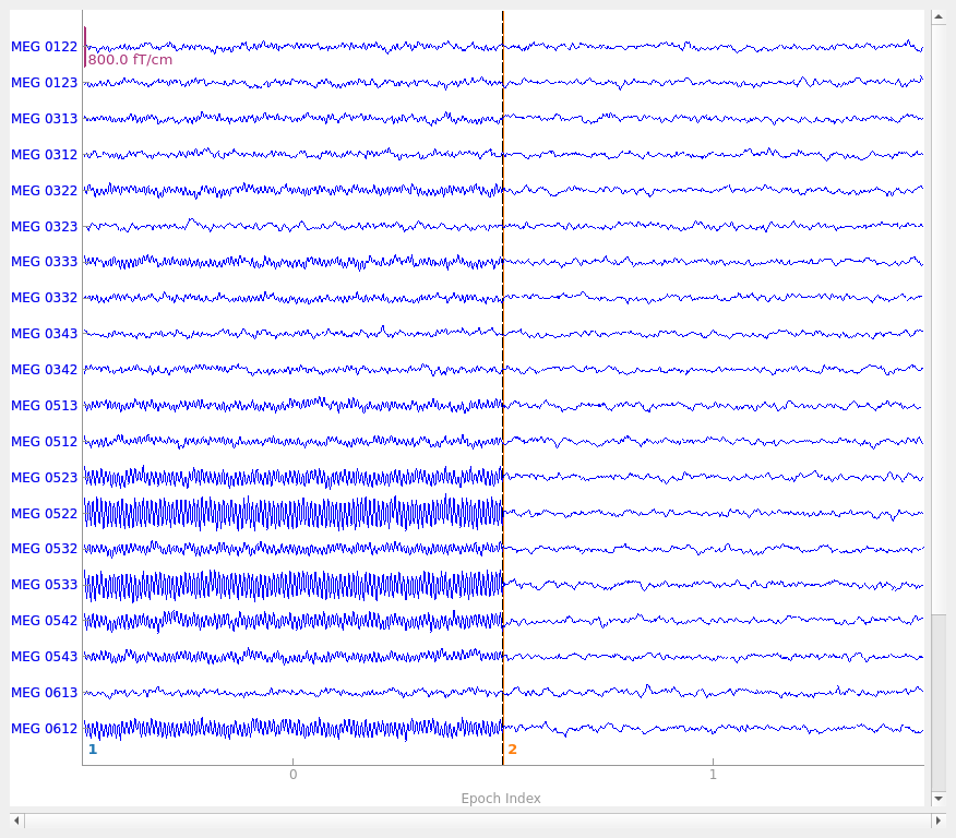
我们创建一个包含两个试次的 mne.Epochs 对象:一个同时包含噪声和信号,另一个仅包含噪声
events = mne.find_events(raw, initial_event=True)
tmax = (len(stc_signal.times) - 1) / sfreq
epochs = mne.Epochs(
    raw,
    events,
    event_id=dict(signal=1, noise=2),
    tmin=0,
    tmax=tmax,
    baseline=None,
    preload=True,
)
assert len(epochs) == 2  # ensure that we got the two expected events

# Plot some of the channels of the simulated data that are situated above one
# of our simulated sources.
picks = mne.read_vectorview_selection("Left-frontal")  # contains both mag and grad
picks = [p for p in picks if p in epochs.ch_names]  # now only grads
epochs.plot(picks=picks, events=True)
Finding events on: STI 014
2 events found on stim channel STI 014
Event IDs: [1 2]
Not setting metadata
2 matching events found
No baseline correction applied
0 projection items activated
Using data from preloaded Raw for 2 events and 500 original time points ...
0 bad epochs dropped
Using qt as 2D backend.
功率映射#
仿真数据集准备就绪后,我们现在可以假装自己是研究者,刚刚从真实受试者身上记录到这些数据,并准备研究大脑的哪些部分彼此通信。
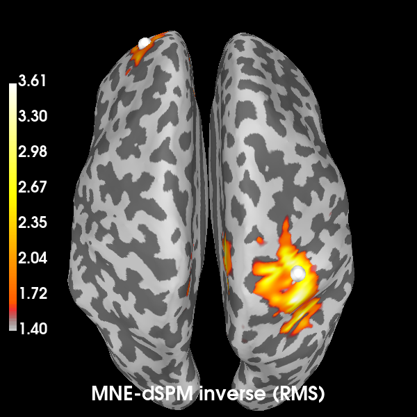
首先,我们将对 MEG 数据创建源估计。为此我们会使用直接的 MNE-dSPM 逆解,以及专为振荡数据设计的 DICS 波束形成器。
使用 MNE-dSPM 计算逆解:
# Compute the inverse operator
fwd = mne.read_forward_solution(fwd_fname)
inv = make_inverse_operator(epochs.info, fwd, cov)

# Apply the inverse model to the trial that also contains the signal.
s = apply_inverse(epochs["signal"].average(), inv)

# Take the root-mean square along the time dimension and plot the result.
s_rms = np.sqrt((s**2).mean())
title = "MNE-dSPM inverse (RMS)"
brain = s_rms.plot(
    "sample",
    subjects_dir=subjects_dir,
    hemi="both",
    figure=1,
    size=600,
    time_label=title,
    title=title,
)

# Indicate the true locations of the source activity on the plot.
brain.add_foci(vertices[0][0], coords_as_verts=True, hemi="lh")
brain.add_foci(vertices[1][0], coords_as_verts=True, hemi="rh")

# Rotate the view and add a title.
brain.show_view(azimuth=0, elevation=0, distance=550, focalpoint=(0, 0, 0))
Reading forward solution from /home/circleci/mne_data/MNE-sample-data/MEG/sample/sample_audvis-meg-eeg-oct-6-fwd.fif...
    Reading a source space...
    Computing patch statistics...
    Patch information added...
    Distance information added...
    [done]
    Reading a source space...
    Computing patch statistics...
    Patch information added...
    Distance information added...
    [done]
    2 source spaces read
    Desired named matrix (kind = 3523 (FIFF_MNE_FORWARD_SOLUTION_GRAD)) not available
    Read MEG forward solution (7498 sources, 306 channels, free orientations)
    Desired named matrix (kind = 3523 (FIFF_MNE_FORWARD_SOLUTION_GRAD)) not available
    Read EEG forward solution (7498 sources, 60 channels, free orientations)
    Forward solutions combined: MEG, EEG
    Source spaces transformed to the forward solution coordinate frame
Converting forward solution to surface orientation
    Average patch normals will be employed in the rotation to the local surface coordinates....
    Converting to surface-based source orientations...
    [done]
Computing inverse operator with 203 channels.
    203 out of 366 channels remain after picking
Selected 203 channels
Creating the depth weighting matrix...
    203 planar channels
    limit = 7262/7498 = 10.020865
    scale = 2.58122e-08 exp = 0.8
Applying loose dipole orientations to surface source spaces: 0.2
Whitening the forward solution.
Computing rank from covariance with rank=None
    Using tolerance 4.5e-14 (2.2e-16 eps * 203 dim * 1  max singular value)
    Estimated rank (grad): 203
    GRAD: rank 203 computed from 203 data channels with 0 projectors
    Setting small GRAD eigenvalues to zero (without PCA)
Creating the source covariance matrix
Adjusting source covariance matrix.
Computing SVD of whitened and weighted lead field matrix.
    largest singular value = 5.59828
    scaling factor to adjust the trace = 2.89697e+18 (nchan = 203 nzero = 0)
Preparing the inverse operator for use...
    Scaled noise and source covariance from nave = 1 to nave = 1
    Created the regularized inverter
    The projection vectors do not apply to these channels.
    Created the whitener using a noise covariance matrix with rank 203 (0 small eigenvalues omitted)
    Computing noise-normalization factors (dSPM)...
[done]
Applying inverse operator to "signal"...
    Picked 203 channels from the data
    Computing inverse...
    Eigenleads need to be weighted ...
    Computing residual...
    Explained  75.6% variance
    Combining the current components...
    dSPM...
[done]
Using control points [1.40954994 1.68061364 3.58897472]
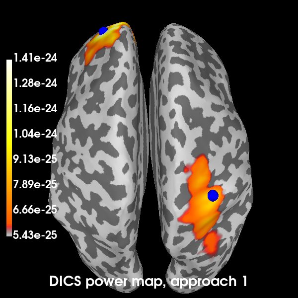
现在我们将使用 DICS 波束形成器计算 10 Hz 的皮层功率图。波束形成器会为每个顶点构建一个空间滤波器,其目标是让源自该顶点的活动通过,同时尽可能抑制来自其他源的活动。
mne.beamformer.make_dics() 函数提供了许多开关,可以精确控制滤波器权重的计算方式。目前,对于哪种方法最佳尚无明确共识。因此,我们将在这里演示两种方法:
# Estimate the cross-spectral density (CSD) matrix on the trial containing the
# signal.
csd_signal = csd_morlet(epochs["signal"], frequencies=[10])

# Compute the spatial filters for each vertex, using two approaches.
filters_approach1 = make_dics(
    info,
    fwd,
    csd_signal,
    reg=0.05,
    pick_ori="max-power",
    depth=1.0,
    inversion="single",
    weight_norm=None,
    real_filter=True,
)
print(filters_approach1)

filters_approach2 = make_dics(
    info,
    fwd,
    csd_signal,
    reg=0.05,
    pick_ori="max-power",
    depth=None,
    inversion="matrix",
    weight_norm="unit-noise-gain",
    real_filter=True,
)
print(filters_approach2)

# You can save these to disk with:
# filters_approach1.save('filters_1-dics.h5')

# Compute the DICS power map by applying the spatial filters to the CSD matrix.
power_approach1, f = apply_dics_csd(csd_signal, filters_approach1)
power_approach2, f = apply_dics_csd(csd_signal, filters_approach2)
Computing cross-spectral density from epochs...

  0%|          | CSD epoch blocks : 0/1 [00:00<?,       ?it/s]
100%|██████████| CSD epoch blocks : 1/1 [00:00<00:00,   71.55it/s]
[done]
Identifying common channels ...
Dropped the following channels:
['MEG 2611', 'MEG 2131', 'MEG 1211', 'MEG 0731', 'STI 001', 'MEG 0721', 'EEG 053', 'STI 016', 'MEG 1041', 'MEG 2431', 'EEG 027', 'MEG 2011', 'MEG 1611', 'MEG 2521', 'EEG 028', 'EEG 017', 'MEG 1841', 'MEG 2621', 'EEG 042', 'EEG 050', 'MEG 0611', 'EEG 007', 'MEG 0631', 'STI 006', 'MEG 1741', 'MEG 1341', 'EEG 012', 'MEG 1111', 'MEG 0411', 'MEG 0141', 'MEG 0231', 'MEG 1811', 'MEG 2121', 'EEG 056', 'STI 005', 'EEG 014', 'EEG 031', 'EEG 026', 'MEG 1541', 'EEG 043', 'EEG 057', 'MEG 2511', 'EEG 052', 'MEG 1931', 'MEG 0521', 'MEG 1711', 'MEG 1131', 'EEG 001', 'MEG 2441', 'MEG 1511', 'MEG 0131', 'MEG 0811', 'MEG 1531', 'EEG 036', 'EEG 011', 'MEG 1721', 'MEG 1441', 'EEG 023', 'MEG 1031', 'MEG 0911', 'MEG 1121', 'EEG 060', 'MEG 1221', 'MEG 1521', 'MEG 1731', 'MEG 0621', 'STI 003', 'EEG 044', 'MEG 1621', 'MEG 2041', 'EEG 018', 'MEG 0241', 'MEG 1641', 'MEG 1021', 'EEG 051', 'MEG 2631', 'EEG 021', 'MEG 2211', 'STI 004', 'MEG 2321', 'EEG 045', 'MEG 2411', 'MEG 0311', 'MEG 2311', 'EEG 030', 'MEG 1421', 'MEG 1311', 'MEG 0431', 'MEG 1411', 'MEG 1831', 'EEG 015', 'MEG 1331', 'EEG 032', 'MEG 2141', 'MEG 2443', 'EEG 055', 'EEG 047', 'EEG 006', 'MEG 2531', 'EEG 025', 'MEG 2641', 'EEG 008', 'EEG 020', 'EEG 005', 'MEG 0921', 'MEG 0441', 'MEG 1631', 'EEG 059', 'MEG 0821', 'MEG 1141', 'EEG 022', 'MEG 0321', 'EEG 049', 'EEG 009', 'MEG 1431', 'EEG 035', 'EEG 039', 'MEG 1911', 'MEG 0111', 'MEG 2331', 'MEG 0641', 'MEG 0341', 'EEG 029', 'MEG 1921', 'MEG 2341', 'EEG 004', 'EEG 040', 'MEG 0421', 'STI 014', 'EEG 002', 'MEG 0121', 'MEG 1941', 'MEG 2031', 'STI 002', 'STI 015', 'MEG 0511', 'MEG 1321', 'MEG 0531', 'MEG 1821', 'MEG 2541', 'MEG 1011', 'EEG 013', 'MEG 1241', 'MEG 0221', 'MEG 2111', 'EEG 058', 'MEG 0211', 'EEG 041', 'EEG 033', 'EEG 038', 'MEG 0741', 'MEG 0331', 'EEG 054', 'MEG 0711', 'MEG 2221', 'EEG 016', 'EEG 034', 'MEG 0931', 'EEG 019', 'MEG 2021', 'MEG 1231', 'EEG 024', 'MEG 2231', 'EEG 037', 'MEG 0541', 'EEG 010', 'EEG 046', 'EEG 048', 'MEG 2421', 'MEG 2241', 'MEG 0941', 'EEG 003']
Computing inverse operator with 203 channels.
    203 out of 203 channels remain after picking
Selected 203 channels
Creating the depth weighting matrix...
Whitening the forward solution.
Computing rank from covariance with rank=None
    Using tolerance 4.5e+08 (2.2e-16 eps * 203 dim * 1e+22  max singular value)
    Estimated rank (grad): 203
    GRAD: rank 203 computed from 203 data channels with 0 projectors
    Setting small GRAD eigenvalues to zero (without PCA)
Creating the source covariance matrix
Adjusting source covariance matrix.
Computing rank from covariance with rank=None
    Using tolerance 1.5e-12 (2.2e-16 eps * 203 dim * 32  max singular value)
    Estimated rank (grad): 138
    GRAD: rank 138 computed from 203 data channels with 0 projectors
Computing DICS spatial filters...
Computing beamformer filters for 7498 sources
Filter computation complete
<Beamformer | DICS, subject "sample", 7498 vert, 203 ch, max-power ori, single inversion>
Identifying common channels ...
Dropped the following channels:
['MEG 2611', 'MEG 2131', 'MEG 1211', 'MEG 0731', 'STI 001', 'MEG 0721', 'EEG 053', 'STI 016', 'MEG 1041', 'MEG 2431', 'EEG 027', 'MEG 2011', 'MEG 1611', 'MEG 2521', 'EEG 028', 'EEG 017', 'MEG 1841', 'MEG 2621', 'EEG 042', 'EEG 050', 'MEG 0611', 'EEG 007', 'MEG 0631', 'STI 006', 'MEG 1741', 'MEG 1341', 'EEG 012', 'MEG 1111', 'MEG 0411', 'MEG 0141', 'MEG 0231', 'MEG 1811', 'MEG 2121', 'EEG 056', 'STI 005', 'EEG 014', 'EEG 031', 'EEG 026', 'MEG 1541', 'EEG 043', 'EEG 057', 'MEG 2511', 'EEG 052', 'MEG 1931', 'MEG 0521', 'MEG 1711', 'MEG 1131', 'EEG 001', 'MEG 2441', 'MEG 1511', 'MEG 0131', 'MEG 0811', 'MEG 1531', 'EEG 036', 'EEG 011', 'MEG 1721', 'MEG 1441', 'EEG 023', 'MEG 1031', 'MEG 0911', 'MEG 1121', 'EEG 060', 'MEG 1221', 'MEG 1521', 'MEG 1731', 'MEG 0621', 'STI 003', 'EEG 044', 'MEG 1621', 'MEG 2041', 'EEG 018', 'MEG 0241', 'MEG 1641', 'MEG 1021', 'EEG 051', 'MEG 2631', 'EEG 021', 'MEG 2211', 'STI 004', 'MEG 2321', 'EEG 045', 'MEG 2411', 'MEG 0311', 'MEG 2311', 'EEG 030', 'MEG 1421', 'MEG 1311', 'MEG 0431', 'MEG 1411', 'MEG 1831', 'EEG 015', 'MEG 1331', 'EEG 032', 'MEG 2141', 'MEG 2443', 'EEG 055', 'EEG 047', 'EEG 006', 'MEG 2531', 'EEG 025', 'MEG 2641', 'EEG 008', 'EEG 020', 'EEG 005', 'MEG 0921', 'MEG 0441', 'MEG 1631', 'EEG 059', 'MEG 0821', 'MEG 1141', 'EEG 022', 'MEG 0321', 'EEG 049', 'EEG 009', 'MEG 1431', 'EEG 035', 'EEG 039', 'MEG 1911', 'MEG 0111', 'MEG 2331', 'MEG 0641', 'MEG 0341', 'EEG 029', 'MEG 1921', 'MEG 2341', 'EEG 004', 'EEG 040', 'MEG 0421', 'STI 014', 'EEG 002', 'MEG 0121', 'MEG 1941', 'MEG 2031', 'STI 002', 'STI 015', 'MEG 0511', 'MEG 1321', 'MEG 0531', 'MEG 1821', 'MEG 2541', 'MEG 1011', 'EEG 013', 'MEG 1241', 'MEG 0221', 'MEG 2111', 'EEG 058', 'MEG 0211', 'EEG 041', 'EEG 033', 'EEG 038', 'MEG 0741', 'MEG 0331', 'EEG 054', 'MEG 0711', 'MEG 2221', 'EEG 016', 'EEG 034', 'MEG 0931', 'EEG 019', 'MEG 2021', 'MEG 1231', 'EEG 024', 'MEG 2231', 'EEG 037', 'MEG 0541', 'EEG 010', 'EEG 046', 'EEG 048', 'MEG 2421', 'MEG 2241', 'MEG 0941', 'EEG 003']
Computing inverse operator with 203 channels.
    203 out of 203 channels remain after picking
Selected 203 channels
Whitening the forward solution.
Computing rank from covariance with rank=None
    Using tolerance 4.5e+08 (2.2e-16 eps * 203 dim * 1e+22  max singular value)
    Estimated rank (grad): 203
    GRAD: rank 203 computed from 203 data channels with 0 projectors
    Setting small GRAD eigenvalues to zero (without PCA)
Creating the source covariance matrix
Adjusting source covariance matrix.
Computing rank from covariance with rank=None
    Using tolerance 1.5e-12 (2.2e-16 eps * 203 dim * 32  max singular value)
    Estimated rank (grad): 138
    GRAD: rank 138 computed from 203 data channels with 0 projectors
Computing DICS spatial filters...
Computing beamformer filters for 7498 sources
Filter computation complete
<Beamformer | DICS, subject "sample", 7498 vert, 203 ch, max-power ori, unit-noise-gain norm, matrix inversion>
Computing DICS source power...
[done]
Computing DICS source power...
[done]
绘制两种方法的 DICS 功率图,先从第一种方法开始:
def plot_approach(power, n):
    """Plot the results on a brain."""
    title = f"DICS power map, approach {n}"
    brain = power_approach1.plot(
        "sample",
        subjects_dir=subjects_dir,
        hemi="both",
        size=600,
        time_label=title,
        title=title,
    )
    # Indicate the true locations of the source activity on the plot.
    brain.add_foci(vertices[0][0], coords_as_verts=True, hemi="lh", color="b")
    brain.add_foci(vertices[1][0], coords_as_verts=True, hemi="rh", color="b")
    # Rotate the view and add a title.
    brain.show_view(azimuth=0, elevation=0, distance=550, focalpoint=(0, 0, 0))
    return brain


brain1 = plot_approach(power_approach1, 1)
Using control points [6.08552772e-25 6.82226119e-25 1.29235324e-24]
现在看第二种方法:
brain2 = plot_approach(power_approach2, 2)
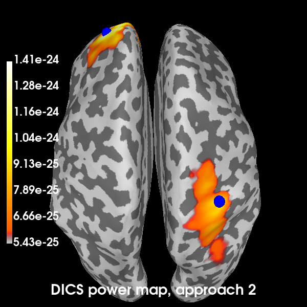
Using control points [6.08552772e-25 6.82226119e-25 1.29235324e-24]
很好!所有方法都找到了我们仿真的两个源。当然,在信噪比(SNR)为 1 的情况下,找到它们并不困难。您可以尝试调整 SNR,看看在噪声不断增大时 MNE-dSPM 和 DICS 方法的表现如何。噪声更大时,您可能需要增大 DICS 波束形成器的正则化参数。
参考文献#
脚本总运行时间:(0 分钟 7.817 秒)