
说明
转到末尾下载完整示例代码。
跨位置泛化(GAL)解码与 TimeGAL#
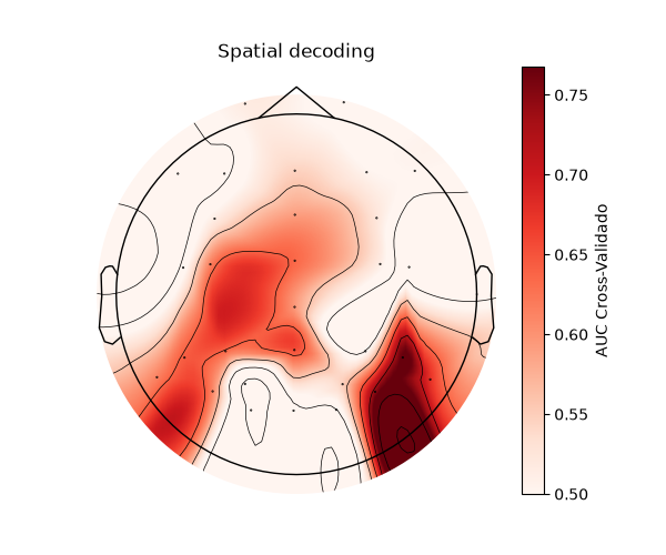
传统上,多变量模式分析(MVPA)或解码技术会在每个单一时间点上使用空间信息(特征)来训练和测试分类器。然而,某些电生理成分在时域中比在空间域中能更好地被捕捉。因此,本教程聚焦于这类时间信息,将其作为训练分类器模型的特征。由此可获得解码率的地形图表示,描绘参与所分析神经成分的脑区位置。
此外,空间解码允许在一个通道上训练分类器模型,并在其他每个通道上进行估计。所得矩阵展示了可解码的时间模式如何在传感器阵列中迁移。跨位置泛化(GAL)流程计算一个通道×通道矩阵,揭示脑区之间的泛化情况。随后可用连接性图来表示交叉解码的泛化模式。这种交叉解码技术类似于 King & Dehaene 提出的时间泛化(参见时间泛化示例),但方向正交:它不展示神经表征在时间上的持续性,而是展示神经表征在不同脑区之间的空间位移。
对于形状为 trials × sensors × time 的 Epochs,时间泛化以时间为迭代轴、以传感器为特征。GAL 将二者的角色对调:传感器位置作为迭代轴,时间采样点作为特征。两种分析都使用 mne.decoding.GeneralizingEstimator。像 GAL 分析这样的空间解码既可在传感器层面进行(适用于 EEG 电极),也可在源层面进行(皮层顶点或 ROI)。在使用 EEG 数据时,强烈建议施加 Laplacian 校正,以避免因容积传导而在邻近区域之间产生虚假的交叉解码泛化。为保持简短并聚焦于解码本身,本教程未对数据施加 Laplacian。
本教程使用 ERP CORE 数据集中的 N170 面孔知觉任务。为加快计算,本教程仅呈现一名被试的数据。我们将面孔与汽车进行对比,并使用 30 个 EEG 传感器。因此,此处展示的结果仅来自单个被试;若要评估哪些 GAL 连接或地形图准确率具有统计显著性,还需要进行跨被试的进一步统计分析。关于 TimeGAL 方法的更多信息可参阅 Santos-Mayo 等人的文章:https://doi.org/10.1002/hbm.70152。
# Authors: The MNE-Python contributors.
# License: BSD-3-Clause
# Copyright the MNE-Python contributors.
下载一个 ERP CORE N170 记录#
ERP CORE 以 BIDS 数据集的形式可从 NEMAR 获取。我们仅下载被试 1(participant 1)的 N170 记录(约 94 MB),而不是完整的多被试存档。该记录包含 80 个面孔试次和 80 个打乱面孔(scrambled face)试次。
import matplotlib.pyplot as plt
import numpy as np
import pooch
from sklearn.linear_model import LogisticRegression
from sklearn.model_selection import StratifiedKFold
from sklearn.pipeline import make_pipeline
from sklearn.preprocessing import StandardScaler

import mne
from mne.channels import make_standard_montage
from mne.decoding import GeneralizingEstimator, SlidingEstimator, cross_val_multiscore
from mne.io import read_raw_eeglab

data_dir = mne.datasets.default_path() / "ERP-CORE-N170" / "sub-001" / "eeg"
data_dir.mkdir(parents=True, exist_ok=True)
urls = {
    "sub-001_task-N170_eeg.fdt": (
        "https://data.nemar.org/nm000132/v1.1.1/sub-001/eeg/sub-001_task-N170_eeg.fdt",
        "sha256:08406f3c6b4a869dc8f67c9acc233a91993bae1b04b7dee5bc0521677ed8949b",
    ),
    "sub-001_task-N170_eeg.set": (
        "https://data.nemar.org/nm000132/v1.1.1/sub-001/eeg/sub-001_task-N170_eeg.set",
        "sha256:9c53dbdc3b469934a5eb6e9f01e59090dd47aeb495b8f21ceca03670991e5b11",
    ),
    "sub-001_task-N170_events.tsv": (
        "https://raw.githubusercontent.com/nemarDatasets/nm000132/v1.1.1/"
        "sub-001/eeg/sub-001_task-N170_events.tsv",
        "sha256:07c87e728d097b0deb05b17d77bbdbd22ef58105111b0b56e659a767b9421e34",
    ),
}
for fname, (url, known_hash) in urls.items():
    pooch.retrieve(url=url, known_hash=known_hash, path=data_dir, fname=fname)

raw = read_raw_eeglab(data_dir / "sub-001_task-N170_eeg.set", preload=True)
Using default location ~/mne_data...
Reading /home/circleci/mne_data/ERP-CORE-N170/sub-001/eeg/sub-001_task-N170_eeg.fdt
Reading 0 ... 699391  =      0.000 ...   682.999 secs...
准备 Epochs#
EEGLAB 记录将三个眼电通道标记为 EEG。在重新参考(re-referencing)之前,先将它们标记为 EOG。为使传感器空间图保持一致,我们使用与记录电极帽标签对应的标准 10-20 位置。全部 30 个头皮电极都参与分析;下面的 picks=\"eeg\" 仅排除 EOG。最后,提取用于解码的 X(试次、传感器、时间)和 y(标签)。
raw.set_channel_types(
    {name: "eog" for name in ("HEOG_left", "HEOG_right", "VEOG_lower")}
)
raw.set_montage(make_standard_montage("colin27_1020"), match_case=False)
raw.filter(0.1, 30.0, fir_design="firwin")
raw.set_eeg_reference(projection=True).apply_proj()

events_tsv = np.genfromtxt(
    data_dir / "sub-001_task-N170_events.tsv",
    delimiter="\t",
    names=True,
    dtype=None,
    encoding="utf-8",
)
is_target_trial = (events_tsv["trial_type"] == "stimulus") & np.isin(
    events_tsv["event_type"], ("face", "scrambled_face")
)
events_tsv = events_tsv[is_target_trial]
event_id = dict(face=1, scrambled_face=2)
events = np.column_stack(
    (
        events_tsv["sample"],
        np.zeros(len(events_tsv), dtype=int),
        np.where(events_tsv["event_type"] == "face", 1, 2),
    )
).astype(int)
epochs = mne.Epochs(
    raw,
    events,
    event_id=event_id,
    tmin=-0.2,
    tmax=0.6,
    baseline=(None, 0),
    picks="eeg",
    preload=True,
    verbose=False,
)
feature_epochs = epochs.copy().crop(0.05, 0.25)
X = feature_epochs.get_data()
y = epochs.events[:, 2] == event_id["face"]
print(
    "Sensor-generalization input: "
    f"{X.shape[0]} trials, {X.shape[1]} scalp sensors, {X.shape[2]} times"
)
Filtering raw data in 1 contiguous segment
Setting up band-pass filter from 0.1 - 30 Hz

FIR filter parameters
---------------------
Designing a one-pass, zero-phase, non-causal bandpass filter:
- Windowed time-domain design (firwin) method
- Hamming window with 0.0194 passband ripple and 53 dB stopband attenuation
- Lower passband edge: 0.10
- Lower transition bandwidth: 0.10 Hz (-6 dB cutoff frequency: 0.05 Hz)
- Upper passband edge: 30.00 Hz
- Upper transition bandwidth: 7.50 Hz (-6 dB cutoff frequency: 33.75 Hz)
- Filter length: 33793 samples (33.001 s)

EEG channel type selected for re-referencing
Adding average EEG reference projection.
1 projection items deactivated
Average reference projection was added, but has not been applied yet. Use the apply_proj method to apply it.
Created an SSP operator (subspace dimension = 1)
1 projection items activated
SSP projectors applied...
Sensor-generalization input: 160 trials, 30 scalp sensors, 206 times
空间分辨解码以时间为特征#
时间分辨解码与空间分辨解码的主要区别在于:什么信息被用作特征(信息),什么被用作迭代轴(滑动)。这里我们介绍空间分辨解码,即分析中使用每个传感器的信息,并将所有时间点作为特征。我们使用 SlidingEstimator 函数,其结果可用地形图展示。需要强调的是,GeneralizingEstimator 默认将最后一个维度(通常是时间)作为迭代轴。设置 axis=1 可选择传感器而非时间,从而将时间解码切换为空间解码。
classifier = make_pipeline(
    StandardScaler(), LogisticRegression(solver="liblinear", random_state=0)
)
cv = StratifiedKFold(n_splits=3, shuffle=True, random_state=0)
space_decoder = SlidingEstimator(
    classifier, scoring="roc_auc", n_jobs=1, verbose=False, axis=1
)
space_scores = cross_val_multiscore(space_decoder, X, y, cv=cv, n_jobs=1).mean(axis=0)


fig, ax = plt.subplots(figsize=(6, 5))
im, _ = mne.viz.plot_topomap(
    space_scores,
    feature_epochs.info,
    axes=ax,
    cmap="Reds",
    vlim=(0.5, None),
    show=False,
)
fig.colorbar(im, ax=ax, label="AUC Cross-Validado")
ax.set_title("Spatial decoding")
plt.show()
跨位置泛化(GAL)#
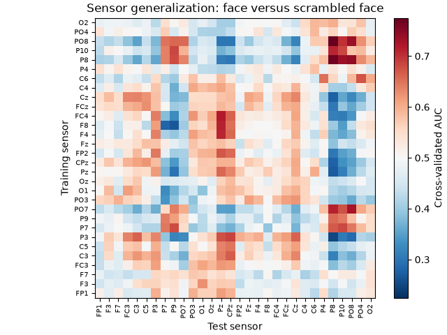
在一个传感器上训练分类器模型,并在其他每个传感器上估计其解码准确率,便得到 GAL 矩阵。这个传感器×传感器矩阵展示了某一传感器或脑区所学习到的条件间差异能在其他皮层区域中被分类的程度。
sensor_gen = GeneralizingEstimator(
    classifier,
    scoring="roc_auc",
    n_jobs=1,
    axis=1,
    verbose=False,
)
对留出试次评分#
三个分层折(stratified fold)分别留出该被试的试次。
scores = []
for train, test in cv.split(X, y):
    scores.append(sensor_gen.fit(X[train], y[train]).score(X[test], y[test]))
scores = np.array(scores)
mean_scores = scores.mean(axis=0)
off_diagonal = ~np.eye(len(epochs.ch_names), dtype=bool)
print(
    "Mean AUC: "
    f"{np.diag(mean_scores).mean():.3f} within sensor; "
    f"{mean_scores[off_diagonal].mean():.3f} across sensors"
)
Mean AUC: 0.551 within sensor; 0.502 across sensors
检查 GAL 交叉解码矩阵#
行对应训练传感器,列对应测试传感器。对角线为传感器内解码,即使用 SlidingWindow 所得到的同一信息(参见上方的地形图)。非对角线单元检验在某一位置学到的时间模式能否在另一位置成立。当两个位置携带相反极性的模式时,可能出现显著的低于机会水平的迁移。需要注意的是,单个被试的矩阵并不构成组水平推断。要确定矩阵中哪些元素具有统计显著性,必须使用所有被试的全部 n 个 GAL 矩阵,针对机会水平(此处为 0.5)进行双侧对比检验。
limit = np.max(np.abs(mean_scores - 0.5))
fig, ax = plt.subplots(layout="constrained")
image = ax.imshow(
    mean_scores,
    origin="lower",
    cmap="RdBu_r",
    vmin=0.5 - limit,
    vmax=0.5 + limit,
    interpolation="nearest",
)
ax.set(
    title="Sensor generalization: face versus scrambled face",
    xlabel="Test sensor",
    ylabel="Training sensor",
)
sensor_ticks = np.arange(len(epochs.ch_names))
ax.set_xticks(sensor_ticks, epochs.ch_names, rotation=90)
ax.set_yticks(sensor_ticks, epochs.ch_names)
ax.tick_params(axis="both", labelsize=7)
fig.colorbar(image, ax=ax, label="Cross-validated AUC")
地形连接性检查#
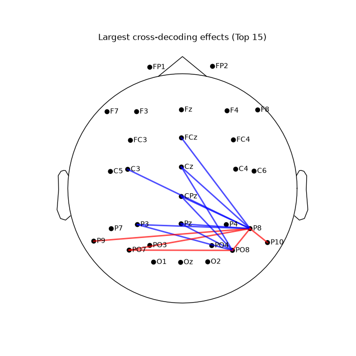
GAL 矩阵的形状与连接矩阵相对应,即传感器×传感器。因此,这些结果可绘制为地形连接图,用以说明哪些脑区似乎表现出相似的神经元响应。为简便起见,仅显示最重要的 15 条连线。蓝线表示那些显示出相似时间模式的交叉解码泛化(显著高于机会水平),红线表示具有相反时间模式的泛化(低于机会水平)。值得注意的是,这只是基于解码的传感器泛化分数展示,而非真实的物理连接图。
cross_sensor_effects = mean_scores - 0.5
cross_sensor_effects = (cross_sensor_effects + cross_sensor_effects.T) / 2

np.fill_diagonal(cross_sensor_effects, 0)
fig, ax = plt.subplots(figsize=(7, 7))
mne.viz.plot_sensors(epochs.info, kind="topomap", show_names=True, axes=ax, show=False)
pos = ax.collections[0].get_offsets()
n_lines = 15
triu_idx = np.triu_indices_from(cross_sensor_effects, k=1)
strongest_vals = np.sort(np.abs(cross_sensor_effects[triu_idx]))
threshold = strongest_vals[-n_lines]
for i in range(len(epochs.ch_names)):
    for j in range(i + 1, len(epochs.ch_names)):
        val = cross_sensor_effects[i, j]

        if abs(val) >= threshold and val != 0:
            x_coords = [pos[i, 0], pos[j, 0]]
            y_coords = [pos[i, 1], pos[j, 1]]

            color = "red" if val > 0 else "blue"

            ax.plot(x_coords, y_coords, color=color, linewidth=2, alpha=0.7)

ax.set_title(f"Largest cross-decoding effects (Top {n_lines})")
plt.show()
使用相关性进行特征重要性分析#
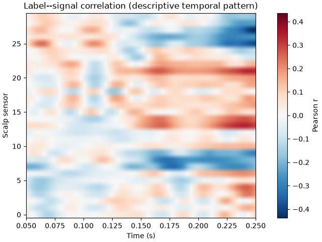
更进一步是估计 Time-GAL 矩阵。Time-GAL 流程将后向解码模型(解码 GAL 矩阵)与前向模型(相关矩阵)配对,从而揭示空间与时间上的泛化连接性。相关矩阵表明条件间差异在何时(时间)与何处(传感器)出现。这里,我们计算二值化的面孔或汽车标签与每个传感器、每个时间点信号之间的 Pearson 相关。由此得到一个通道×时间的相关矩阵。
X_centered = X - X.mean(axis=0)
y_centered = y - y.mean()
label_signal_correlation = np.einsum("n,nct->ct", y_centered, X_centered)
label_signal_correlation /= np.sqrt(
    np.sum(y_centered**2) * np.sum(X_centered**2, axis=0)
)
corr_limit = np.max(np.abs(label_signal_correlation))
fig, ax = plt.subplots(layout="constrained")
image = ax.imshow(
    label_signal_correlation,
    aspect="auto",
    cmap="RdBu_r",
    extent=(
        feature_epochs.times[0],
        feature_epochs.times[-1],
        -0.5,
        len(epochs.ch_names) - 0.5,
    ),
    origin="lower",
    vmin=-corr_limit,
    vmax=corr_limit,
)
ax.set(
    title="Label--signal correlation (descriptive temporal pattern)",
    xlabel="Time (s)",
    ylabel="Scalp sensor",
)
fig.colorbar(image, ax=ax, label="Pearson r")
结合时间信息与 GAL 连接性#
要获得 Time-GAL 信息,需要将 GAL 解码信息与相关矩阵的信息配对。为合并这两个矩阵,首先必须根据其与机会水平(GAL)或 0(Pearson 相关)的距离,将矩阵阈值化为显著或相关的信息。在计算完每名被试的矩阵后,可通过找出统计显著的元素来获得该阈值。然而,在本单被试教程中,我们仅选取 GAL 矩阵中大于 0.6 或小于 0.4 的元素,以及 ±0.25 的元素。合并后得到一个传感器×传感器×时间的三维矩阵,其中 0 表示缺乏任何相关信息,而数值表示特定时间点上两个区域或传感器之间 GAL 连接的强度。
relevant_timechannels = np.abs(label_signal_correlation) > 0.25
relevant_GAL = ((mean_scores - 0.5) > 0.1) + -1 * ((mean_scores - 0.5) < -0.1)

timeGAL = np.zeros(
    (relevant_GAL.shape[0], relevant_GAL.shape[1], relevant_timechannels.shape[1])
)
for i in range(relevant_GAL.shape[0]):
    for j in range(relevant_GAL.shape[0]):
        if relevant_GAL[i, j] != 0:
            timeGAL[i, j, :] = (mean_scores[i, j] - 0.5) * (
                relevant_timechannels[i, :] * np.abs(label_signal_correlation[i, :])
            )
在地形图与大脑上展示 TimeGAL 模式#
最后,Time-GAL 模式可以按时间片段展示。这里我们将试次时段分为 5 个时间窗,展示 GAL 连接模式如何随时间演变。它描绘了面孔与汽车知觉过程中脑区相互作用的时空表征。
times_ms = feature_epochs.times * 1000
fig, axes = plt.subplots(1, 5, figsize=(20, 4), layout="constrained")

for k, ax in enumerate(axes):
    i0, i1 = k * 41, (k + 1) * 41
    wGAL = timeGAL[:, :, i0:i1].mean(axis=2)

    mne.viz.plot_sensors(
        epochs.info, kind="topomap", show_names=False, axes=ax, show=False
    )
    pos = ax.collections[0].get_offsets()

    triu = np.triu_indices_from(wGAL, k=1)
    vals_abs = np.abs(wGAL[triu])
    thresh, max_v = np.sort(vals_abs)[-15], vals_abs.max()

    for i in range(len(epochs.ch_names)):
        for j in range(i + 1, len(epochs.ch_names)):
            val = wGAL[i, j]
            if abs(val) >= thresh and val != 0:
                nw = (abs(val) - thresh) / (max_v - thresh + 1e-10)
                ax.plot(
                    pos[[i, j], 0],
                    pos[[i, j], 1],
                    color="red" if val > 0 else "blue",
                    linewidth=1 + 4 * nw,
                    alpha=0.3 + 0.7 * nw,
                )

    ax.set_title(f"Time {times_ms[i0]:.0f} to {times_ms[i1 - 1]:.0f} ms")

plt.show()
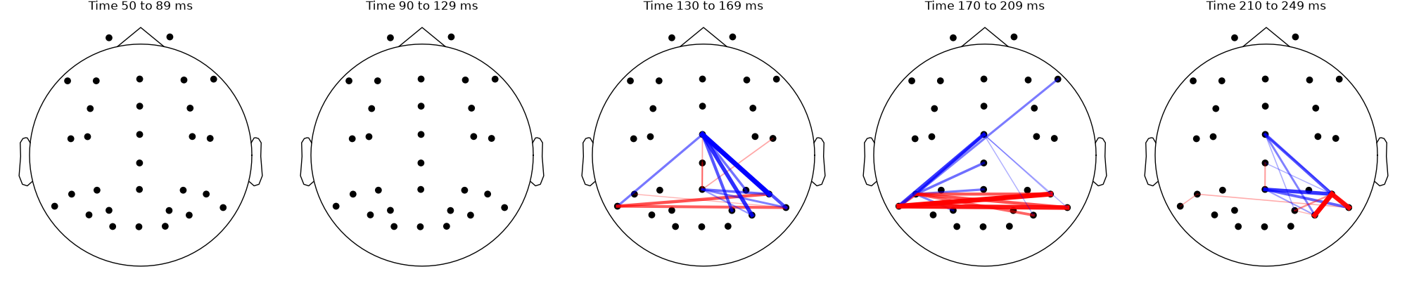
组水平统计与显著结果#
本教程演示了空间解码、GAL 与 TimeGAL 流程的估计方法。然而,它只展示了 ERP-CORE 数据集中第一名被试的 EEG 活动。因此,结果仅反映单个被试的解码情况,无法计算统计显著性。理想情况下,应对实验样本中的每名被试分别计算该分析。当完成整个组的计算并提取数据后,可将每名被试的地形图、GAL 矩阵与 Pearson 相关矩阵作为分布,用于配对检验(例如 Student's T 检验),以分别衡量其与机会水平或 0 的统计差异。值得注意的是,这些统计分析必须进行族系错误率(FWER)校正,例如置换检验或 Bonferroni 校正,以确保解码结果准确且稳健。
关于 Time-GAL 方法的更多细节可参阅其原始文章:Santos-Mayo et al. (2025) Decoding in the Fourth Dimension: Classification of Temporal Patterns and Their Generalization Across Locations - https://doi.org/10.1002/hbm.70152
脚本总运行时间:(0 分钟 5.006 秒)