非官方中文翻译 本页译自 MNE-Python 官方文档： 查看英文原文 ↗。 文档版权归 MNE Developers 所有（BSD-3-Clause）。

使用 MNE、dSPM、sLORETA 和 eLORETA 进行源定位

本教程旨在教你如何对诱发数据、原始数据和 Epochs 数据计算并应用线性最小范数逆方法。

# Authors: The MNE-Python contributors.
# License: BSD-3-Clause
# Copyright the MNE-Python contributors.

import matplotlib.pyplot as plt
import numpy as np

import mne
from mne.datasets import sample
from mne.minimum_norm import apply_inverse, make_inverse_operator

处理 MEG 数据

data_path = sample.data_path()
raw_fname = data_path / "MEG" / "sample" / "sample_audvis_filt-0-40_raw.fif"

raw = mne.io.read_raw_fif(raw_fname)  # already has an average reference
events = mne.find_events(raw, stim_channel="STI 014")

event_id = dict(aud_l=1)  # event trigger and conditions
tmin = -0.2  # start of each epoch (200ms before the trigger)
tmax = 0.5  # end of each epoch (500ms after the trigger)
raw.info["bads"] = ["MEG 2443", "EEG 053"]  # mark known bad channels
baseline = (None, 0)  # means from the first instant to t = 0
reject = dict(grad=4000e-13, mag=4e-12, eog=150e-6)

epochs = mne.Epochs(
    raw,
    events,
    event_id,
    tmin,
    tmax,
    proj=True,
    picks=("meg", "eog"),
    baseline=baseline,
    reject=reject,
)

Opening raw data file /home/circleci/mne_data/MNE-sample-data/MEG/sample/sample_audvis_filt-0-40_raw.fif...
    Read a total of 4 projection items:
        PCA-v1 (1 x 102)  idle
        PCA-v2 (1 x 102)  idle
        PCA-v3 (1 x 102)  idle
        Average EEG reference (1 x 60)  idle
    Range : 6450 ... 48149 =     42.956 ...   320.665 secs
Ready.
Finding events on: STI 014
319 events found on stim channel STI 014
Event IDs: [ 1  2  3  4  5 32]
Not setting metadata
72 matching events found
Setting baseline interval to [-0.19979521315838786, 0.0] s
Applying baseline correction (mode: mean)
Created an SSP operator (subspace dimension = 3)
3 projection items activated

计算正则化噪声协方差

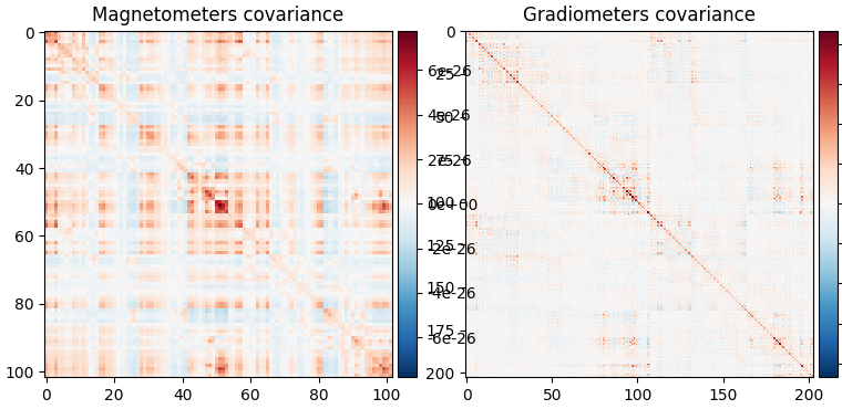
更多细节请参阅 计算协方差矩阵。

noise_cov = mne.compute_covariance(
    epochs, tmax=0.0, method=["shrunk", "empirical"], rank=None, verbose=True
)

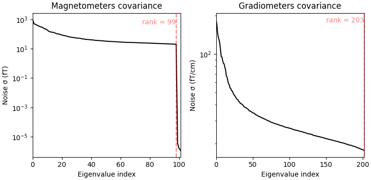
fig_cov, fig_spectra = mne.viz.plot_cov(noise_cov, raw.info)

• 
• 

Loading data for 72 events and 106 original time points ...
    Rejecting  epoch based on EOG : ['EOG 061']
    Rejecting  epoch based on EOG : ['EOG 061']
    Rejecting  epoch based on EOG : ['EOG 061']
    Rejecting  epoch based on EOG : ['EOG 061']
    Rejecting  epoch based on EOG : ['EOG 061']
    Rejecting  epoch based on MAG : ['MEG 1711']
    Rejecting  epoch based on EOG : ['EOG 061']
    Rejecting  epoch based on EOG : ['EOG 061']
    Rejecting  epoch based on EOG : ['EOG 061']
    Rejecting  epoch based on EOG : ['EOG 061']
    Rejecting  epoch based on EOG : ['EOG 061']
    Rejecting  epoch based on EOG : ['EOG 061']
    Rejecting  epoch based on EOG : ['EOG 061']
    Rejecting  epoch based on EOG : ['EOG 061']
    Rejecting  epoch based on EOG : ['EOG 061']
    Rejecting  epoch based on EOG : ['EOG 061']
    Rejecting  epoch based on EOG : ['EOG 061']
17 bad epochs dropped
    Created an SSP operator (subspace dimension = 3)
    Setting small MEG eigenvalues to zero (without PCA)
Reducing data rank from 305 -> 302
Estimating covariance using SHRUNK
Done.
Estimating covariance using EMPIRICAL
Done.
Using cross-validation to select the best estimator.
Number of samples used : 1705
log-likelihood on unseen data (descending order):
   shrunk: -1466.423
   empirical: -1574.608
selecting best estimator: shrunk
[done]
Computing rank from covariance with rank=None
    Using tolerance 2.2e-14 (2.2e-16 eps * 102 dim * 0.98  max singular value)
    Estimated rank (mag): 99
    MAG: rank 99 computed from 102 data channels with 0 projectors
Computing rank from covariance with rank=None
    Using tolerance 1.6e-13 (2.2e-16 eps * 203 dim * 3.5  max singular value)
    Estimated rank (grad): 203
    GRAD: rank 203 computed from 203 data channels with 0 projectors

计算诱发响应

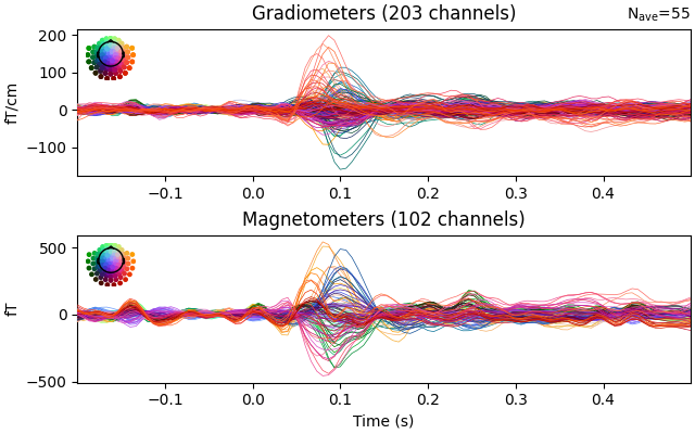
为简单起见，我们只使用 MEG 通道。

evoked = epochs.average().pick("meg")
evoked.plot(time_unit="s")
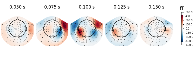
evoked.plot_topomap(times=np.linspace(0.05, 0.15, 5), ch_type="mag")

• 
• 

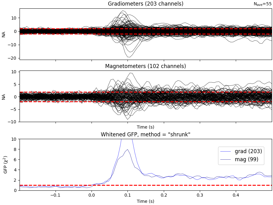
查看白化后的数据也是个好主意：

evoked.plot_white(noise_cov, time_unit="s")
del epochs, raw  # to save memory

NOTE: pick_types() is a legacy function. New code should use inst.pick(...).
Computing rank from covariance with rank=None
    Using tolerance 1.6e-13 (2.2e-16 eps * 203 dim * 3.5  max singular value)
    Estimated rank (grad): 203
    GRAD: rank 203 computed from 203 data channels with 0 projectors
Computing rank from covariance with rank=None
    Using tolerance 2.2e-14 (2.2e-16 eps * 102 dim * 0.98  max singular value)
    Estimated rank (mag): 99
    MAG: rank 99 computed from 102 data channels with 3 projectors
    Created an SSP operator (subspace dimension = 3)
Computing rank from covariance with rank={'grad': 203, 'mag': 99, 'meg': 302}
    Setting small MEG eigenvalues to zero (without PCA)
    Created the whitener using a noise covariance matrix with rank 302 (3 small eigenvalues omitted)

逆建模：对诱发数据与原始数据应用 MNE/dSPM

这里我们首先读取正向解。对于你自己的数据，你很可能需要计算一个正向解——具体做法参见 头模型与正向计算。

fname_fwd = data_path / "MEG" / "sample" / "sample_audvis-meg-oct-6-fwd.fif"
fwd = mne.read_forward_solution(fname_fwd)

Reading forward solution from /home/circleci/mne_data/MNE-sample-data/MEG/sample/sample_audvis-meg-oct-6-fwd.fif...
    Reading a source space...
    Computing patch statistics...
    Patch information added...
    Distance information added...
    [done]
    Reading a source space...
    Computing patch statistics...
    Patch information added...
    Distance information added...
    [done]
    2 source spaces read
    Desired named matrix (kind = 3523 (FIFF_MNE_FORWARD_SOLUTION_GRAD)) not available
    Read MEG forward solution (7498 sources, 306 channels, free orientations)
    Source spaces transformed to the forward solution coordinate frame

接下来，我们构建一个 MEG 逆算子。

inverse_operator = make_inverse_operator(
    evoked.info, fwd, noise_cov, loose=0.2, depth=0.8
)
del fwd

Converting forward solution to surface orientation
    Average patch normals will be employed in the rotation to the local surface coordinates....
    Converting to surface-based source orientations...
    [done]
info["bads"] and noise_cov["bads"] do not match, excluding bad channels from both
Computing inverse operator with 305 channels.
    305 out of 306 channels remain after picking
Selected 305 channels
Creating the depth weighting matrix...
    203 planar channels
    limit = 7265/7498 = 10.037795
    scale = 2.52065e-08 exp = 0.8
Applying loose dipole orientations to surface source spaces: 0.2
Whitening the forward solution.
    Created an SSP operator (subspace dimension = 3)
Computing rank from covariance with rank=None
    Using tolerance 2.9e-13 (2.2e-16 eps * 305 dim * 4.2  max singular value)
    Estimated rank (mag + grad): 302
    MEG: rank 302 computed from 305 data channels with 3 projectors
    Setting small MEG eigenvalues to zero (without PCA)
Creating the source covariance matrix
Adjusting source covariance matrix.
Computing SVD of whitened and weighted lead field matrix.
    largest singular value = 4.69746
    scaling factor to adjust the trace = 8.82367e+18 (nchan = 305 nzero = 3)

说明

你可以用下面的方式将逆算子写入磁盘：

from mne.minimum_norm import write_inverse_operator
write_inverse_operator(
    "sample_audvis-meg-oct-6-inv.fif", inverse_operator
)

计算逆解

我们可以用它计算逆解，从而获得源时间过程：

method = "dSPM"  # could choose MNE, sLORETA, or eLORETA instead
snr = 3.0
lambda2 = 1.0 / snr**2
stc, residual = apply_inverse(
    evoked,
    inverse_operator,
    lambda2,
    method=method,
    pick_ori=None,
    return_residual=True,
    verbose=True,
)

Preparing the inverse operator for use...
    Scaled noise and source covariance from nave = 1 to nave = 55
    Created the regularized inverter
    Created an SSP operator (subspace dimension = 3)
    Created the whitener using a noise covariance matrix with rank 302 (3 small eigenvalues omitted)
    Computing noise-normalization factors (dSPM)...
[done]
Applying inverse operator to "aud_l"...
    Picked 305 channels from the data
    Computing inverse...
    Eigenleads need to be weighted ...
    Computing residual...
    Explained  66.0% variance
    Combining the current components...
    dSPM...
[done]

可视化

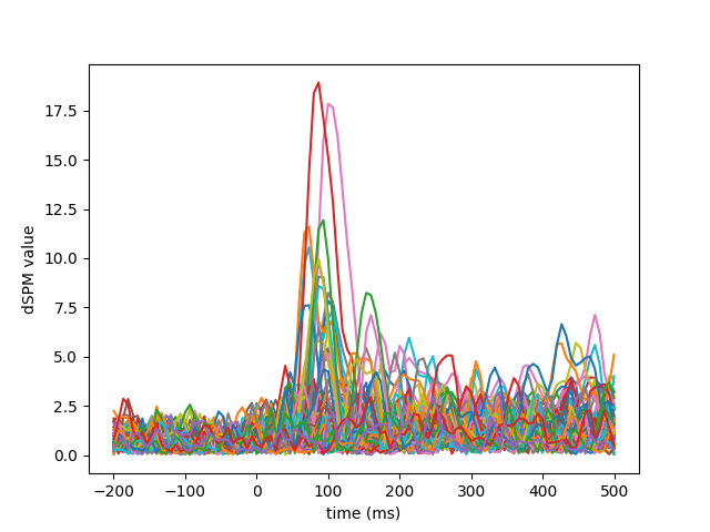
我们可以查看不同的偶极子激活：

fig, ax = plt.subplots()
ax.plot(1e3 * stc.times, stc.data[::100, :].T)
ax.set(xlabel="time (ms)", ylabel=f"{method} value")

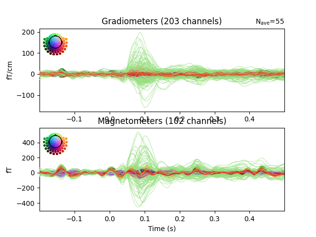
检查原始数据以及拟合后的残差：

fig, axes = plt.subplots(2, 1)
evoked.plot(axes=axes)
for ax in axes:
    for text in list(ax.texts):
        text.remove()
    for line in ax.lines:
        line.set_color("#98df81")
residual.plot(axes=axes)

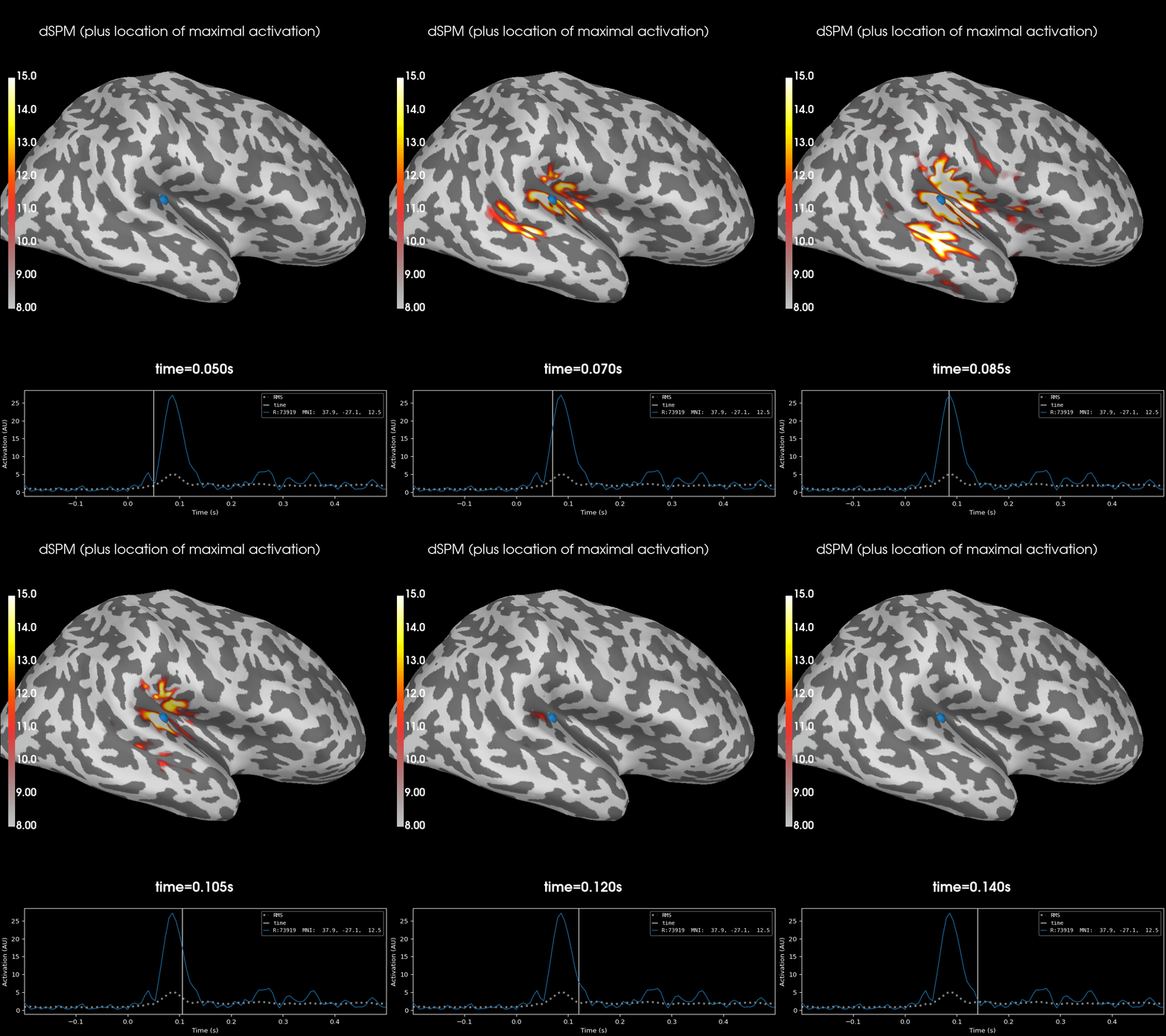
这里我们使用 get_peak 将可视化移动到峰值所在的时间点，并在峰值最大的顶点处绘制标记。

vertno_max, time_max = stc.get_peak(hemi="rh")

subjects_dir = data_path / "subjects"
surfer_kwargs = dict(
    hemi="rh",
    subjects_dir=subjects_dir,
    clim=dict(kind="value", lims=[8, 12, 15]),
    views="lateral",
    initial_time=time_max,
    time_unit="s",
    size=(800, 800),
    smoothing_steps=10,
)
brain = stc.plot(**surfer_kwargs)
brain.add_foci(
    vertno_max,
    coords_as_verts=True,
    hemi="rh",
    color="blue",
    scale_factor=0.6,
    alpha=0.5,
)
brain.add_text(
    0.1, 0.9, "dSPM (plus location of maximal activation)", "title", font_size=14
)

# The documentation website's movie is generated with:
# brain.save_movie(..., tmin=0.05, tmax=0.15, interpolation='linear',
#                  time_dilation=20, framerate=10, time_viewer=True)

还有许多其他可视化和处理源数据的方法，例如：

• 可视化源时间过程（STC）

• 变换皮层表面源估计

• 变换体积源估计

• 绘制完整的向量值 MNE 解

• 偶极子方向在分布式源定位中的作用

• 计算多种 MNE 解

• 使用 apply_inverse 的示例。