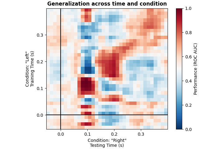
传感器空间解码：跨时间与条件的泛化#

本示例运行 [1] 中描述的分析。它展示如何拟合一个线性分类器，在给定时点找出具有判别性的地形图，随后评估该线性模型能否准确预测另一组条件的所有时间采样点。

# Authors: Jean-Rémi King <jeanremi.king@gmail.com>
#          Alexandre Gramfort <alexandre.gramfort@inria.fr>
#          Denis Engemann <denis.engemann@gmail.com>
#
# License: BSD-3-Clause
# Copyright the MNE-Python contributors.

import matplotlib.pyplot as plt
from sklearn.linear_model import LogisticRegression
from sklearn.pipeline import make_pipeline
from sklearn.preprocessing import StandardScaler

import mne
from mne.datasets import sample
from mne.decoding import GeneralizingEstimator

# Preprocess data
data_path = sample.data_path()
# Load and filter data, set up epochs
meg_path = data_path / "MEG" / "sample"
raw_fname = meg_path / "sample_audvis_filt-0-40_raw.fif"
events_fname = meg_path / "sample_audvis_filt-0-40_raw-eve.fif"
raw = mne.io.read_raw_fif(raw_fname, preload=True)
picks = mne.pick_types(raw.info, meg=True, exclude="bads")  # Pick MEG channels
raw.filter(1.0, 30.0, fir_design="firwin")  # Band pass filtering signals
events = mne.read_events(events_fname)
event_id = {
    "Auditory/Left": 1,
    "Auditory/Right": 2,
    "Visual/Left": 3,
    "Visual/Right": 4,
}
tmin = -0.050
tmax = 0.400
# decimate to make the example faster to run, but then use verbose='error' in
# the Epochs constructor to suppress warning about decimation causing aliasing
decim = 2
epochs = mne.Epochs(
    raw,
    events,
    event_id=event_id,
    tmin=tmin,
    tmax=tmax,
    proj=True,
    picks=picks,
    baseline=None,
    preload=True,
    reject=dict(mag=5e-12),
    decim=decim,
    verbose="error",
)

Opening raw data file /home/circleci/mne_data/MNE-sample-data/MEG/sample/sample_audvis_filt-0-40_raw.fif...
    Read a total of 4 projection items:
        PCA-v1 (1 x 102)  idle
        PCA-v2 (1 x 102)  idle
        PCA-v3 (1 x 102)  idle
        Average EEG reference (1 x 60)  idle
    Range : 6450 ... 48149 =     42.956 ...   320.665 secs
Ready.
Reading 0 ... 41699  =      0.000 ...   277.709 secs...
Filtering raw data in 1 contiguous segment
Setting up band-pass filter from 1 - 30 Hz

FIR filter parameters
---------------------
Designing a one-pass, zero-phase, non-causal bandpass filter:
- Windowed time-domain design (firwin) method
- Hamming window with 0.0194 passband ripple and 53 dB stopband attenuation
- Lower passband edge: 1.00
- Lower transition bandwidth: 1.00 Hz (-6 dB cutoff frequency: 0.50 Hz)
- Upper passband edge: 30.00 Hz
- Upper transition bandwidth: 7.50 Hz (-6 dB cutoff frequency: 33.75 Hz)
- Filter length: 497 samples (3.310 s)

我们在所有左侧视觉 vs 听觉试次上训练分类器，并在所有右侧视觉 vs 听觉试次上测试。

clf = make_pipeline(
    StandardScaler(),
    # liblinear is faster than lbfgs
    LogisticRegression(solver="liblinear", random_state=131),
)
time_gen = GeneralizingEstimator(clf, scoring="roc_auc", n_jobs=None, verbose=True)

# Fit classifiers on the epochs where the stimulus was presented to the left.
# Note that the experimental condition y indicates auditory or visual
time_gen.fit(X=epochs["Left"].get_data(copy=False), y=epochs["Left"].events[:, 2] > 2)

  0%|          | Fitting GeneralizingEstimator : 0/35 [00:00<?,       ?it/s]
 14%|█▍        | Fitting GeneralizingEstimator : 5/35 [00:00<00:00,  148.07it/s]
 34%|███▍      | Fitting GeneralizingEstimator : 12/35 [00:00<00:00,  178.62it/s]
 54%|█████▍    | Fitting GeneralizingEstimator : 19/35 [00:00<00:00,  189.09it/s]
 74%|███████▍  | Fitting GeneralizingEstimator : 26/35 [00:00<00:00,  194.33it/s]
 91%|█████████▏| Fitting GeneralizingEstimator : 32/35 [00:00<00:00,  190.94it/s]
100%|██████████| Fitting GeneralizingEstimator : 35/35 [00:00<00:00,  194.80it/s]

<GeneralizingEstimator(base_estimator=Pipeline(steps=[('standardscaler', StandardScaler()), ('logisticregression', LogisticRegression(random_state=131, solver='liblinear'))]), scoring='roc_auc', verbose=True, fitted with 35 estimators, fitted with 35 estimators>

In a Jupyter environment, please rerun this cell to show the HTML representation or trust the notebook.
On GitHub, the HTML representation is unable to render, please try loading this page with nbviewer.org.

GeneralizingEstimator

iFitted

Parameters

	base_estimator	Pipeline(step...liblinear'))])
	scoring	'roc_auc'
	verbose	True
	n_jobs	None
	position	0
	allow_2d	False
	axis	-1

Fitted attributes

Name	Type	Value
classes_	ndarray[bool](2,)	[False, True]
estimators_	ndarray[object](35,)	[Pipeline(steps=[('standardscaler', StandardScaler()), ('logisticregression', LogisticRegression(random_state=131, solver='liblinear'))]), Pipeline(steps=[('standardscaler', StandardScaler()), ('logisticregression', LogisticRegression(random_state=131, solver='liblinear'))]), Pipeline(steps=[('standardscaler', StandardScaler()), ('logisticregression', LogisticRegression(random_state=131, solver='liblinear'))]), ..., Pipeline(steps=[('standardscaler', StandardScaler()), ('logisticregression', LogisticRegression(random_state=131, solver='liblinear'))]), Pipeline(steps=[('standardscaler', StandardScaler()), ('logisticregression', LogisticRegression(random_state=131, solver='liblinear'))]), Pipeline(steps=[('standardscaler', StandardScaler()), ('logisticregression', LogisticRegression(random_state=131, solver='liblinear'))])]
fit_params_	dict	{}
n_features_in_	int	305

base_estimator: Pipeline

StandardScaler

?Documentation for StandardScaler

Parameters

	copy copy: bool, default=True If False, try to avoid a copy and do inplace scaling instead. This is not guaranteed to always work inplace; e.g. if the data is not a NumPy array or scipy.sparse CSR matrix, a copy may still be returned.	True
	with_mean with_mean: bool, default=True If True, center the data before scaling. This does not work (and will raise an exception) when attempted on sparse matrices, because centering them entails building a dense matrix which in common use cases is likely to be too large to fit in memory.	True
	with_std with_std: bool, default=True If True, scale the data to unit variance (or equivalently, unit standard deviation).	True

LogisticRegression

?Documentation for LogisticRegression

Parameters

	random_state random_state: int, RandomState instance, default=None Only used for `solver` == 'sag', 'saga' or 'liblinear' to shuffle the data. It has no effect on the other solvers. See :term:`Glossary <random_state>` for details.	131
	solver solver: {'lbfgs', 'liblinear', 'newton-cg', 'newton-cholesky', 'sag', 'saga'}, default='lbfgs' Algorithm to use in the optimization problem. Default is 'lbfgs'. To choose a solver, you might want to consider the following aspects: - 'lbfgs' is a good default solver because it works reasonably well for a wide class of problems. - For :term:`multiclass` problems (`n_classes >= 3`), all solvers except 'liblinear' minimize the full multinomial loss, 'liblinear' will raise an error. - 'newton-cholesky' is a good choice for `n_samples` >> `n_features * n_classes`, especially with one-hot encoded categorical features with rare categories. Be aware that the memory usage of this solver has a quadratic dependency on `n_features * n_classes` because it explicitly computes the full Hessian matrix. - For small datasets, 'liblinear' is a good choice, whereas 'sag' and 'saga' are faster for large ones; - 'liblinear' can only handle binary classification by default. To apply a one-versus-rest scheme for the multiclass setting one can wrap it with the :class:`~sklearn.multiclass.OneVsRestClassifier`. .. warning:: The choice of the algorithm depends on the penalty chosen (`l1_ratio=0` for L2-penalty, `l1_ratio=1` for L1-penalty and `0 < l1_ratio < 1` for Elastic-Net) and on (multinomial) multiclass support: ================= ======================== ====================== solver l1_ratio multinomial multiclass ================= ======================== ====================== 'lbfgs' l1_ratio=0 yes 'liblinear' l1_ratio=1 or l1_ratio=0 no 'newton-cg' l1_ratio=0 yes 'newton-cholesky' l1_ratio=0 yes 'sag' l1_ratio=0 yes 'saga' 0<=l1_ratio<=1 yes ================= ======================== ====================== .. note:: 'sag' and 'saga' fast convergence is only guaranteed on features with approximately the same scale. You can preprocess the data with a scaler from :mod:`sklearn.preprocessing`. .. seealso:: Refer to the :ref:`User Guide <Logistic_regression>` for more information regarding :class:`LogisticRegression` and more specifically the :ref:`Table <logistic_regression_solvers>` summarizing solver/penalty supports. .. versionadded:: 0.17 Stochastic Average Gradient (SAG) descent solver. Multinomial support in version 0.18. .. versionadded:: 0.19 SAGA solver. .. versionchanged:: 0.22 The default solver changed from 'liblinear' to 'lbfgs' in 0.22. .. versionadded:: 1.2 newton-cholesky solver. Multinomial support in version 1.6.	'liblinear'
	penalty penalty: {'l1', 'l2', 'elasticnet', None}, default='l2' Specify the norm of the penalty: - `None`: no penalty is added; - `'l2'`: add an L2 penalty term and it is the default choice; - `'l1'`: add an L1 penalty term; - `'elasticnet'`: both L1 and L2 penalty terms are added. .. warning:: Some penalties may not work with some solvers. See the parameter `solver` below, to know the compatibility between the penalty and solver. .. versionadded:: 0.19 l1 penalty with SAGA solver (allowing 'multinomial' + L1) .. deprecated:: 1.8 `penalty` was deprecated in version 1.8 and will be removed in 1.10. Use `l1_ratio` and `C` instead. `l1_ratio=0` for `penalty='l2'`, `l1_ratio=1` for `penalty='l1'`, `l1_ratio` set to any float between 0 and 1 for `penalty='elasticnet'`, and `C=np.inf` for `penalty=None`.	'deprecated'
	C C: float, default=1.0 Inverse of regularization strength; must be a positive float. Like in support vector machines, smaller values specify stronger regularization. `C=np.inf` results in unpenalized logistic regression. For a visual example on the effect of tuning the `C` parameter with an L1 penalty, see: :ref:`sphx_glr_auto_examples_linear_model_plot_logistic_path.py`.	1.0
	l1_ratio l1_ratio: float, default=0.0 The Elastic-Net mixing parameter, with `0 <= l1_ratio <= 1`. Setting `l1_ratio=1` gives a pure L1-penalty, setting `l1_ratio=0` a pure L2-penalty. Any value between 0 and 1 gives an Elastic-Net penalty of the form `l1_ratio * L1 + (1 - l1_ratio) * L2`. .. warning:: Certain values of `l1_ratio`, i.e. some penalties, may not work with some solvers. See the parameter `solver` below, to know the compatibility between the penalty and solver. .. versionchanged:: 1.8 Default value changed from None to 0.0. .. deprecated:: 1.8 `None` is deprecated and will be removed in version 1.10. Always use `l1_ratio` to specify the penalty type.	0.0
	dual dual: bool, default=False Dual (constrained) or primal (regularized, see also :ref:`this equation <regularized-logistic-loss>`) formulation. Dual formulation is only implemented for l2 penalty with liblinear solver. Prefer `dual=False` when n_samples > n_features.	False
	tol tol: float, default=1e-4 Tolerance for stopping criteria.	0.0001
	fit_intercept fit_intercept: bool, default=True Specifies if a constant (a.k.a. bias or intercept) should be added to the decision function.	True
	intercept_scaling intercept_scaling: float, default=1 Useful only when the solver `liblinear` is used and `self.fit_intercept` is set to `True`. In this case, `x` becomes `[x, self.intercept_scaling]`, i.e. a "synthetic" feature with constant value equal to `intercept_scaling` is appended to the instance vector. The intercept becomes ``intercept_scaling * synthetic_feature_weight``. .. note:: The synthetic feature weight is subject to L1 or L2 regularization as all other features. To lessen the effect of regularization on synthetic feature weight (and therefore on the intercept) `intercept_scaling` has to be increased.	1
	class_weight class_weight: dict or 'balanced', default=None Weights associated with classes in the form ``{class_label: weight}``. If not given, all classes are supposed to have weight one. The "balanced" mode uses the values of y to automatically adjust weights inversely proportional to class frequencies in the input data as ``n_samples / (n_classes * np.bincount(y))``. Note that these weights will be multiplied with sample_weight (passed through the fit method) if sample_weight is specified. .. versionadded:: 0.17 class_weight='balanced'	None
	max_iter max_iter: int, default=100 Maximum number of iterations taken for the solvers to converge.	100
	verbose verbose: int, default=0 For the liblinear and lbfgs solvers set verbose to any positive number for verbosity.	0
	warm_start warm_start: bool, default=False When set to True, reuse the solution of the previous call to fit as initialization, otherwise, just erase the previous solution. Useless for liblinear solver. See :term:`the Glossary <warm_start>`. .. versionadded:: 0.17 warm_start to support lbfgs, newton-cg, sag, saga solvers.	False
	n_jobs n_jobs: int, default=None Does not have any effect. .. deprecated:: 1.8 `n_jobs` is deprecated in version 1.8 and will be removed in 1.10.	None

在刺激呈现在右侧的分段上计算得分。

scores = time_gen.score(
    X=epochs["Right"].get_data(copy=False), y=epochs["Right"].events[:, 2] > 2
)

0%|          | Scoring GeneralizingEstimator : 0/1225 [00:00<?,       ?it/s]
1%|          | Scoring GeneralizingEstimator : 11/1225 [00:00<00:03,  325.98it/s]
2%|▏         | Scoring GeneralizingEstimator : 23/1225 [00:00<00:03,  341.69it/s]
3%|▎         | Scoring GeneralizingEstimator : 35/1225 [00:00<00:03,  347.06it/s]
3%|▎         | Scoring GeneralizingEstimator : 35/1225 [00:00<00:03,  335.57it/s]

绘图

fig, ax = plt.subplots(layout="constrained")
im = ax.matshow(
    scores,
    vmin=0,
    vmax=1.0,
    cmap="RdBu_r",
    origin="lower",
    extent=epochs.times[[0, -1, 0, -1]],
)
ax.axhline(0.0, color="k")
ax.axvline(0.0, color="k")
ax.xaxis.set_ticks_position("bottom")
ax.set_xlabel(
    'Condition: "Right"\nTesting Time (s)',
)
ax.set_ylabel('Condition: "Left"\nTraining Time (s)')
ax.set_title("Generalization across time and condition", fontweight="bold")
fig.colorbar(im, ax=ax, label="Performance (ROC AUC)")
plt.show()

Generalization across time and condition

参考文献#

图库由 Sphinx-Gallery 生成