
说明
转到末尾下载完整示例代码。
使用 LIMO 数据集进行单试次线性回归分析#
这里探索 LIMO 数据集 中包含的数据结构。本示例复现并扩展了 LIMO MEEG 中集成的部分主要分析与工具;LIMO MEEG 是一个最初为对接 EEGLAB 而设计的 MATLAB 工具箱。
概括而言,本示例会:
获取 LIMO 数据集 [1] 中单个受试者的分段数据文件。若本地找不到 LIMO 文件,获取函数
mne.datasets.limo.load_data()会自动从远程仓库下载。导入过程中,会从磁盘上的 LIMO
.mat文件中提取数据信息(如采样率、各条件的分段数、每个受试者的 EEG 通道数量与名称等),并作为元数据加入 epochs 结构。在单个受试者的数据上拟合线性模型,并可视化推断指标,以评估所估计效应的显著性。
# Authors: Jose C. Garcia Alanis <alanis.jcg@gmail.com>
#
# License: BSD-3-Clause
# Copyright the MNE-Python contributors.
import matplotlib.pyplot as plt
import numpy as np

from mne import combine_evoked
from mne.datasets.limo import load_data
from mne.stats import linear_regression
from mne.viz import plot_compare_evokeds, plot_events

print(__doc__)

# subject to use
subj = 1
关于数据#
在原始 LIMO 实验(见 [2])中,被试执行二选一强迫选择任务,对两张面孔刺激进行辨别。整个实验使用同样的两张面孔,并加入不同程度的噪声,使面孔对被试而言更易或更难辨认(类似方法见 [3] 图 1)。
呈现的面孔沿噪声—信号(或相位一致性)连续体变化,范围从 0 到 85%,以 5% 为步长递增。换言之,相位一致性高(如 85%)的面孔容易识别,而相位一致性低(如 5%)的面孔难以识别,也就更难辨别。
加载数据#
首先加载 LIMO 数据集中第 1 名受试者的数据。
# This step can take a little while if you're loading the data for the
# first time.
limo_epochs = load_data(subject=subj)
注意,加载结果是 mne.EpochsArray,其中的数据已可直接与 MNE-Python 对接。
print(limo_epochs)
<EpochsArray | 1055 events (all good), -0.3 – 0.5 s (baseline off), ~213.7 MiB, data loaded, with metadata,
 'Face/A': 524
 'Face/B': 531>
可视化事件#
我们可以可视化 limo_epochs 结构中面孔事件的分布。由于分段按条件排序,事件应呈现清晰的分组。
fig = plot_events(limo_epochs.events, event_id=limo_epochs.event_id)
fig.suptitle("Distribution of events in LIMO epochs")
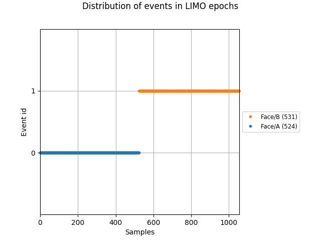
如上所示,条件编码为 Face/A 与 Face/B。所呈现面孔的相位一致性信息保存在 epochs 元数据中,可通过 limo_epochs.metadata 方便地访问。如下所示,元数据还包含所呈现面孔的信息,便于使用。
print(limo_epochs.metadata.head())
  face  phase-coherence
0    A         0.491210
1    A        -1.235572
2    A        -1.043707
3    A         1.642398
4    A        -0.659978
现在进一步查看 epochs 元数据中的信息。
# We want include all columns in the summary table
epochs_summary = limo_epochs.metadata.describe(include="all").round(3)
print(epochs_summary)
        face  phase-coherence
count   1055         1055.000
unique     2              NaN
top        B              NaN
freq     531              NaN
mean     NaN           -0.000
std      NaN            1.000
min      NaN           -1.619
25%      NaN           -0.852
50%      NaN           -0.084
75%      NaN            0.875
max      NaN            1.642
上表第一列提供的信息与之前运行的 print(limo_epochs) 大致相同:共有 1055 个面孔(即分段),分为 2 个条件(Face A 与 Face B);对该受试者而言,Face B 条件的分段更多。
此外,第二列显示相位一致性变量的取值范围为 -1.619 到 1.642。这是因为 LIMO 数据集以 z 分数形式提供相位一致性数值,其均值为 0、标准差为 1。
可视化各条件的 ERP#
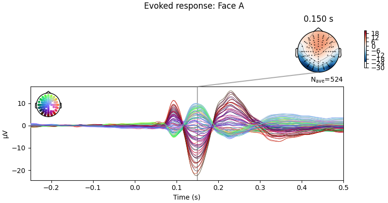
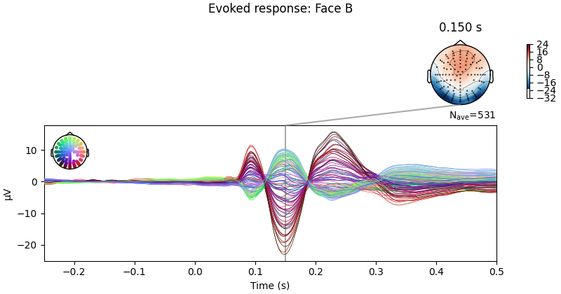
绘制 Face A 与 Face B 诱发的 ERP,看看二者有多相似。
# only show -250 to 500 ms
ts_args = dict(xlim=(-0.25, 0.5))

# plot evoked response for face A
limo_epochs["Face/A"].average().plot_joint(
    times=[0.15], title="Evoked response: Face A", ts_args=ts_args
)
# and face B
limo_epochs["Face/B"].average().plot_joint(
    times=[0.15], title="Evoked response: Face B", ts_args=ts_args
)
No projector specified for this dataset. Please consider the method self.add_proj.
No projector specified for this dataset. Please consider the method self.add_proj.
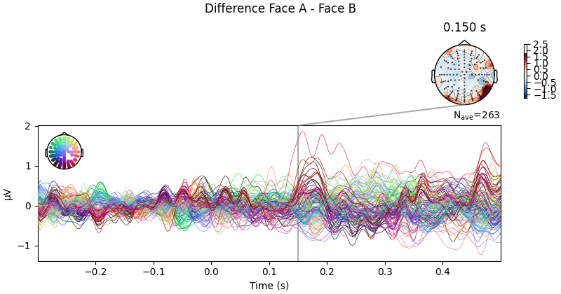
也可以计算对比 Face A 与 Face B 的差异波。不过从上面的诱发响应看,这两种面孔刺激之间不应有太大差异。
# Face A minus Face B
difference_wave = combine_evoked(
    [limo_epochs["Face/A"].average(), limo_epochs["Face/B"].average()], weights=[1, -1]
)

# plot difference wave
difference_wave.plot_joint(times=[0.15], title="Difference Face A - Face B")
No projector specified for this dataset. Please consider the method self.add_proj.
正如预期,对比 Face A 与 Face B 时没有出现明显模式。不过还可以进一步缩小范围:由于这是“视觉范式”,最好查看枕叶附近的电极,因为刺激差异(若有)在视觉区更容易观察到。
# Create a dictionary containing the evoked responses
conditions = ["Face/A", "Face/B"]
evokeds = {condition: limo_epochs[condition].average() for condition in conditions}

# concentrate analysis an occipital electrodes (e.g. B11)
pick = evokeds["Face/A"].ch_names.index("B11")

# compare evoked responses
plot_compare_evokeds(evokeds, picks=pick, ylim=dict(eeg=(-15, 7.5)))
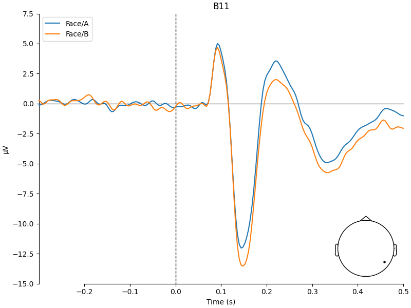
我们确实看到 Face A 与 Face B 之间存在差异,但幅度很小。
可视化刺激相位一致性的效应#
由于相位一致性决定面孔刺激是否容易识别,可以预期相位一致性高的面孔会在枕叶电极上诱发更强的激活模式。
phase_coh = limo_epochs.metadata["phase-coherence"]
# get levels of phase coherence
levels = sorted(phase_coh.unique())
# create labels for levels of phase coherence (i.e., 0 - 85%)
labels = [f"{i:.2f}" for i in np.arange(0.0, 0.90, 0.05)]

# create dict of evokeds for each level of phase-coherence
evokeds = {
    label: limo_epochs[phase_coh == level].average()
    for level, label in zip(levels, labels)
}

# pick channel to plot
electrodes = ["C22", "B11"]
# create figures
for electrode in electrodes:
    fig, ax = plt.subplots(figsize=(8, 4))
    plot_compare_evokeds(
        evokeds,
        axes=ax,
        ylim=dict(eeg=(-20, 15)),
        picks=electrode,
        cmap=("Phase coherence", "magma"),
    )
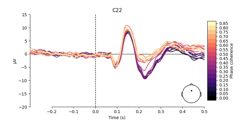
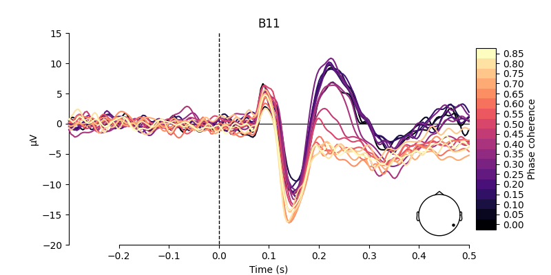
如上所示,在所选电极上,低相位一致性与高相位一致性刺激诱发的激活模式存在明显差异。
为线性回归分析准备数据#
在用线性回归检验这些差异的显著性之前,我们先对预处理阶段被剔除的缺失通道进行插值;此外,还会剔除数据中以“EXG”为前缀的 EOG 通道:
limo_epochs.interpolate_bads(reset_bads=True)
limo_epochs.drop_channels(["EXG1", "EXG2", "EXG3", "EXG4"])
Setting channel interpolation method to {'eeg': 'spline'}.
Interpolating bad channels.
    Automatic origin fit: head of radius 95.0 mm
Computing interpolation matrix from 113 sensor positions
Interpolating 15 sensors
定义预测变量与设计矩阵#
运行回归分析需要构建设计矩阵,其中包含用于预测脑活动模式的变量(即预测变量)。为此,我们使用 limo_epochs.metadata 中的信息:相位一致性以及 Face A 与 Face B 的对比。
# name of predictors + intercept
predictor_vars = ["face a - face b", "phase-coherence", "intercept"]

# create design matrix
design = limo_epochs.metadata[["phase-coherence", "face"]].copy()
design["face a - face b"] = np.where(design["face"] == "A", 1, -1)
design["intercept"] = 1
design = design[predictor_vars]
现在可以使用 MNE-Python 的 linear_regression() 函数建立分析所用的线性模型。
reg = linear_regression(limo_epochs, design_matrix=design, names=predictor_vars)
Fitting linear model to epochs, (25728 targets, 3 regressors)
Done
提取回归系数#
结果保存在对象 reg 中;它是一个由诱发对象组成的字典,为设计矩阵中的每个预测变量提供多种推断指标。
predictors are: ['face a - face b', 'phase-coherence', 'intercept']
fields are: ['beta', 'stderr', 't_val', 'p_val', 'mlog10_p_val']
绘制模型结果#
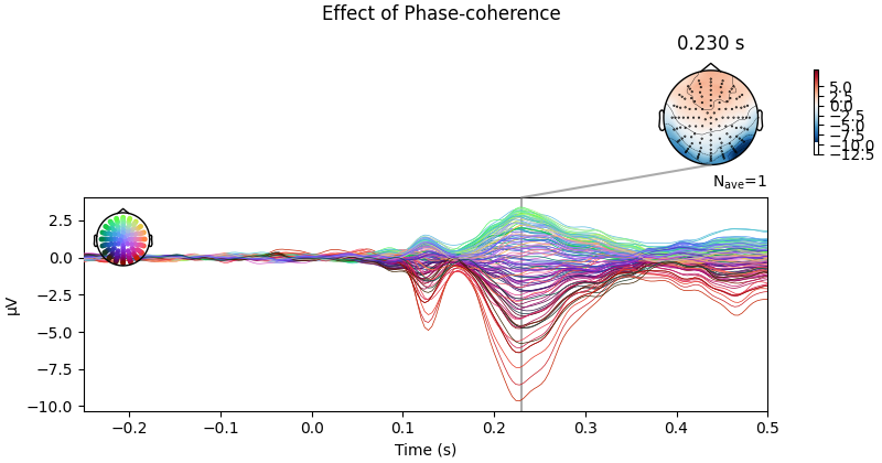
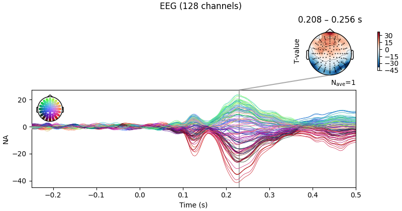
现在可以通过 reg['<name of predictor>'].<measure of interest> 访问并绘制线性回归结果,并像使用其他诱发对象一样调用 plot_joint()。下图可见明显的相位一致性效应:相位一致性越高(即“面孔可见性”越好),刺激后约 200 至 250 ms 枕叶电极测得的活动越呈负向变化。
No projector specified for this dataset. Please consider the method self.add_proj.
也可以绘制相应的 T 值。
# use unit=False and scale=1 to keep values at their original
# scale (i.e., avoid conversion to micro-volt).
ts_args = dict(xlim=(-0.25, 0.5), unit=False)
topomap_args = dict(scalings=dict(eeg=1), average=0.05)

fig = reg["phase-coherence"].t_val.plot_joint(
    ts_args=ts_args, topomap_args=topomap_args, times=[0.23]
)
fig.axes[0].set_ylabel("T-value")
No projector specified for this dataset. Please consider the method self.add_proj.
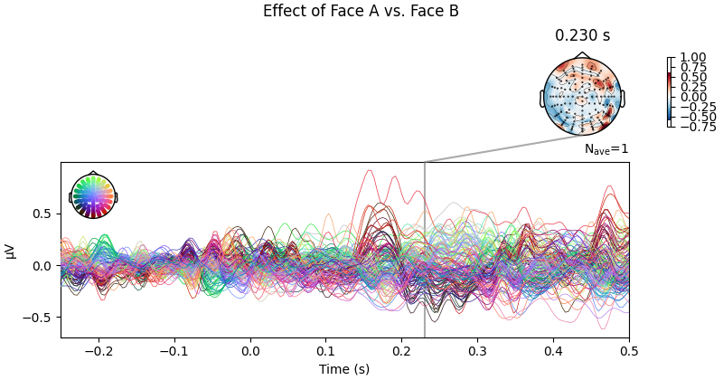
相反,比较 Face A 与 Face B 刺激时似乎没有(或仅有很小的)系统性效应,这与前文的差异波分析基本一致。
No projector specified for this dataset. Please consider the method self.add_proj.
参考文献#
脚本总运行时间:(0 分 6.044 秒)