
非官方中文翻译
本页译自 MNE-Python 官方文档:
查看英文原文 ↗。
文档版权归 MNE Developers 所有(BSD-3-Clause)。
说明
转到末尾下载完整示例代码。
比较模拟与估计的源活动#
本示例说明如何通过计算不同指标来比较模拟与估计的源时间过程(STC)。模拟源可以是皮层区域或偶极子。本示例仅作简要介绍,只展示最简单的用法。
# Author: Kostiantyn Maksymenko <kostiantyn.maksymenko@gmail.com>
#
# License: BSD-3-Clause
# Copyright the MNE-Python contributors.

from functools import partial

import matplotlib.pyplot as plt
import numpy as np

import mne
from mne.datasets import sample
from mne.minimum_norm import apply_inverse, make_inverse_operator
from mne.simulation.metrics import (
    cosine_score,
    f1_score,
    peak_position_error,
    precision_score,
    recall_score,
    region_localization_error,
    spatial_deviation_error,
)

random_state = 229  # set random state to make this example deterministic

# Import sample data
data_path = sample.data_path()
subjects_dir = data_path / "subjects"
subject = "sample"
evoked_fname = data_path / "MEG" / subject / "sample_audvis-ave.fif"
info = mne.io.read_info(evoked_fname)
tstep = 1.0 / info["sfreq"]

# Import forward operator and source space
fwd_fname = data_path / "MEG" / subject / "sample_audvis-meg-eeg-oct-6-fwd.fif"
fwd = mne.read_forward_solution(fwd_fname)
src = fwd["src"]

# To select source, we use the caudal middle frontal to grow
# a region of interest.
selected_label = mne.read_labels_from_annot(
    subject, regexp="caudalmiddlefrontal-lh", subjects_dir=subjects_dir
)[0]
    Read a total of 4 projection items:
        PCA-v1 (1 x 10²) active
        PCA-v2 (1 x 10²) active
        PCA-v3 (1 x 10²) active
        Average EEG reference (1 x 60) active
Reading forward solution from /home/circleci/mne_data/MNE-sample-data/MEG/sample/sample_audvis-meg-eeg-oct-6-fwd.fif...
    Reading a source space...
    Computing patch statistics...
    Patch information added...
    Distance information added...
    [done]
    Reading a source space...
    Computing patch statistics...
    Patch information added...
    Distance information added...
    [done]
    2 source spaces read
    Desired named matrix (kind = 3523 (FIFF_MNE_FORWARD_SOLUTION_GRAD)) not available
    Read MEG forward solution (7498 sources, 306 channels, free orientations)
    Desired named matrix (kind = 3523 (FIFF_MNE_FORWARD_SOLUTION_GRAD)) not available
    Read EEG forward solution (7498 sources, 60 channels, free orientations)
    Forward solutions combined: MEG, EEG
    Source spaces transformed to the forward solution coordinate frame
Reading labels from parcellation...
   read 1 labels from /home/circleci/mne_data/MNE-sample-data/subjects/sample/label/lh.aparc.annot
   read 0 labels from /home/circleci/mne_data/MNE-sample-data/subjects/sample/label/rh.aparc.annot
本示例模拟两类皮层源:区域源与偶极子源,并检验相应的性能指标。
定义源的主要参数#
首先从“何处”“什么”“何时”三个方面定义区域源与偶极子源。
# WHERE?

# Region
location = "center"  # Use the center of the label as a seed.
extent = 20.0  # Extent in mm of the region.
label_region = mne.label.select_sources(
    subject,
    selected_label,
    location=location,
    extent=extent,
    subjects_dir=subjects_dir,
    rng=random_state,
)

# Dipole
location = 1915  # Use the index of the vertex as a seed
extent = 0.0  # One dipole source
label_dipole = mne.label.select_sources(
    subject,
    selected_label,
    location=location,
    extent=extent,
    subjects_dir=subjects_dir,
    rng=random_state,
)

# WHAT?
# Define the time course of the activity
source_time_series = np.sin(2.0 * np.pi * 18.0 * np.arange(100) * tstep) * 10e-9

# WHEN?
# Define when the activity occurs using events.
n_events = 50
events = np.zeros((n_events, 3), int)
events[:, 0] = 200 * np.arange(n_events)  # Events sample.
events[:, 2] = 1  # All events have the sample id.
创建模拟的源活动#
这里使用 SourceSimulator。
# Region
source_simulator_region = mne.simulation.SourceSimulator(src, tstep=tstep)
source_simulator_region.add_data(label_region, source_time_series, events)

# Dipole
source_simulator_dipole = mne.simulation.SourceSimulator(src, tstep=tstep)
source_simulator_dipole.add_data(label_dipole, source_time_series, events)
模拟原始数据#
把源时间序列投影到传感器空间,并加入由示例数据噪声协方差得到的多变量高斯噪声。
# Region
raw_region = mne.simulation.simulate_raw(info, source_simulator_region, forward=fwd)
raw_region = raw_region.pick(picks=["eeg", "stim"], exclude="bads")
cov = mne.make_ad_hoc_cov(raw_region.info)
mne.simulation.add_noise(
    raw_region, cov, iir_filter=[0.2, -0.2, 0.04], rng=random_state
)

# Dipole
raw_dipole = mne.simulation.simulate_raw(info, source_simulator_dipole, forward=fwd)
raw_dipole = raw_dipole.pick(picks=["eeg", "stim"], exclude="bads")
cov = mne.make_ad_hoc_cov(raw_dipole.info)
mne.simulation.add_noise(
    raw_dipole, cov, iir_filter=[0.2, -0.2, 0.04], rng=random_state
)
Setting up raw simulation: 1 position, "cos2" interpolation
Event information stored on channel:              STI 014
    Interval 0.000–1.665 s
Setting up forward solutions
Computing gain matrix for transform #1/1
    Interval 0.000–1.665 s
    Interval 0.000–1.665 s
    Interval 0.000–1.665 s
    Interval 0.000–1.665 s
    Interval 0.000–1.665 s
    Interval 0.000–1.665 s
    Interval 0.000–1.665 s
    Interval 0.000–1.665 s
    Interval 0.000–1.498 s
    10 STC iterations provided
[done]
Adding noise to 59/68 channels (59 channels in cov)
从原始数据计算诱发响应#
对与事件对应的分段进行平均。
# Region
events = mne.find_events(raw_region, initial_event=True)
tmax = (len(source_time_series) - 1) * tstep
epochs = mne.Epochs(raw_region, events, 1, tmin=0, tmax=tmax, baseline=None)
evoked_region = epochs.average()

# Dipole
events = mne.find_events(raw_dipole, initial_event=True)
tmax = (len(source_time_series) - 1) * tstep
epochs = mne.Epochs(raw_dipole, events, 1, tmin=0, tmax=tmax, baseline=None)
evoked_dipole = epochs.average()
Finding events on: STI 014
50 events found on stim channel STI 014
Event IDs: [1]
Not setting metadata
50 matching events found
No baseline correction applied
Created an SSP operator (subspace dimension = 1)
1 projection items activated
Finding events on: STI 014
50 events found on stim channel STI 014
Event IDs: [1]
Not setting metadata
50 matching events found
No baseline correction applied
Created an SSP operator (subspace dimension = 1)
1 projection items activated
创建与诱发响应对应的真实 STC#
此前我们计算了与原始数据对应的 STC。为了与基于诱发响应的重建结果比较,真实 STC 应具有相同的时间采样点数。
# Region
stc_true_region = source_simulator_region.get_stc(
    start_sample=0, stop_sample=len(source_time_series)
)

# Dipole
stc_true_dipole = source_simulator_dipole.get_stc(
    start_sample=0, stop_sample=len(source_time_series)
)
重建模拟的源#
使用 sLORETA 计算逆解。
# Region
snr = 30.0
inv_method = "sLORETA"
lambda2 = 1.0 / snr**2

inverse_operator = make_inverse_operator(
    evoked_region.info, fwd, cov, loose="auto", depth=0.8, fixed=True
)

stc_est_region = apply_inverse(
    evoked_region, inverse_operator, lambda2, inv_method, pick_ori=None
)

# Dipole
snr = 3.0
inv_method = "sLORETA"
lambda2 = 1.0 / snr**2

inverse_operator = make_inverse_operator(
    evoked_dipole.info, fwd, cov, loose="auto", depth=0.8, fixed=True
)

stc_est_dipole = apply_inverse(
    evoked_dipole, inverse_operator, lambda2, inv_method, pick_ori=None
)
Computing inverse operator with 59 channels.
    59 out of 366 channels remain after picking
Selected 59 channels
Creating the depth weighting matrix...
    59 EEG channels
    limit = 7499/7498 = 2.118742
    scale = 155292 exp = 0.8
    Picked elements from a free-orientation depth-weighting prior into the fixed-orientation one
    Average patch normals will be employed in the rotation to the local surface coordinates....
    Converting to surface-based source orientations...
    [done]
Whitening the forward solution.
    Created an SSP operator (subspace dimension = 1)
Computing rank from covariance with rank=None
    Using tolerance 5.2e-18 (2.2e-16 eps * 59 dim * 0.0004  max singular value)
    Estimated rank (eeg): 58
    EEG: rank 58 computed from 59 data channels with 1 projector
    Setting small EEG eigenvalues to zero (without PCA)
Creating the source covariance matrix
Adjusting source covariance matrix.
Computing SVD of whitened and weighted lead field matrix.
    largest singular value = 4.2931
    scaling factor to adjust the trace = 1.34986e+22 (nchan = 59 nzero = 1)
Preparing the inverse operator for use...
    Scaled noise and source covariance from nave = 1 to nave = 50
    Created the regularized inverter
    Created an SSP operator (subspace dimension = 1)
    Created the whitener using a noise covariance matrix with rank 58 (1 small eigenvalues omitted)
    Computing noise-normalization factors (sLORETA)...
[done]
Applying inverse operator to "1"...
    Picked 59 channels from the data
    Computing inverse...
    Eigenleads need to be weighted ...
    Computing residual...
    Explained 100.0% variance
    sLORETA...
[done]
Computing inverse operator with 59 channels.
    59 out of 366 channels remain after picking
Selected 59 channels
Creating the depth weighting matrix...
    59 EEG channels
    limit = 7499/7498 = 2.118742
    scale = 155292 exp = 0.8
    Picked elements from a free-orientation depth-weighting prior into the fixed-orientation one
    Average patch normals will be employed in the rotation to the local surface coordinates....
    Converting to surface-based source orientations...
    [done]
Whitening the forward solution.
    Created an SSP operator (subspace dimension = 1)
Computing rank from covariance with rank=None
    Using tolerance 5.2e-18 (2.2e-16 eps * 59 dim * 0.0004  max singular value)
    Estimated rank (eeg): 58
    EEG: rank 58 computed from 59 data channels with 1 projector
    Setting small EEG eigenvalues to zero (without PCA)
Creating the source covariance matrix
Adjusting source covariance matrix.
Computing SVD of whitened and weighted lead field matrix.
    largest singular value = 4.2931
    scaling factor to adjust the trace = 1.34986e+22 (nchan = 59 nzero = 1)
Preparing the inverse operator for use...
    Scaled noise and source covariance from nave = 1 to nave = 50
    Created the regularized inverter
    Created an SSP operator (subspace dimension = 1)
    Created the whitener using a noise covariance matrix with rank 58 (1 small eigenvalues omitted)
    Computing noise-normalization factors (sLORETA)...
[done]
Applying inverse operator to "1"...
    Picked 59 channels from the data
    Computing inverse...
    Eigenleads need to be weighted ...
    Computing residual...
    Explained  85.1% variance
    sLORETA...
[done]
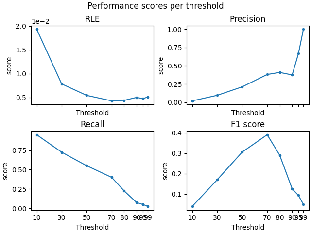
计算不同源幅度阈值下的性能评分#
thresholds = [10, 30, 50, 70, 80, 90, 95, 99]
针对区域#
# create a set of scorers
scorers = {
    "RLE": partial(region_localization_error, src=src),
    "Precision": precision_score,
    "Recall": recall_score,
    "F1 score": f1_score,
}

# compute results
region_results = {}
for name, scorer in scorers.items():
    region_results[name] = [
        scorer(stc_true_region, stc_est_region, threshold=f"{thx}%", per_sample=False)
        for thx in thresholds
    ]

# Plot the results
f, ((ax1, ax2), (ax3, ax4)) = plt.subplots(2, 2, sharex="col", layout="constrained")
for ax, (title, results) in zip([ax1, ax2, ax3, ax4], region_results.items()):
    ax.plot(thresholds, results, ".-")
    ax.set(title=title, ylabel="score", xlabel="Threshold", xticks=thresholds)

f.suptitle("Performance scores per threshold")  # Add Super title
ax1.ticklabel_format(axis="y", style="sci", scilimits=(0, 1))  # tweak RLE

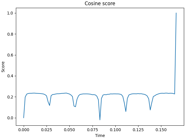
# Cosine score with respect to time
f, ax1 = plt.subplots(layout="constrained")
ax1.plot(stc_true_region.times, cosine_score(stc_true_region, stc_est_region))
ax1.set(title="Cosine score", xlabel="Time", ylabel="Score")
针对偶极子#
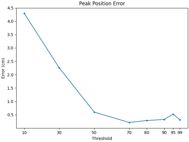
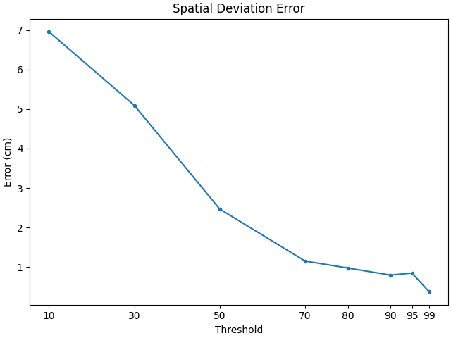
# create a set of scorers
scorers = {
    "Peak Position Error": peak_position_error,
    "Spatial Deviation Error": spatial_deviation_error,
}


# compute results
dipole_results = {}
for name, scorer in scorers.items():
    dipole_results[name] = [
        scorer(
            stc_true_dipole,
            stc_est_dipole,
            src=src,
            threshold=f"{thx}%",
            per_sample=False,
        )
        for thx in thresholds
    ]


# Plot the results
for name, results in dipole_results.items():
    f, ax1 = plt.subplots(layout="constrained")
    ax1.plot(thresholds, 100 * np.array(results), ".-")
    ax1.set(title=name, ylabel="Error (cm)", xlabel="Threshold", xticks=thresholds)
脚本总运行时间:(0 分 2.437 秒)