感受野估计与预测#

本示例复现 Lalor 等人 MATLAB mTRF 工具箱中的图 [1]，展示 mne.decoding.ReceptiveField 类如何结合 scikit-learn 完成类似功能。我们先拟合一个线性编码模型，用连续变化的语音包络预测 128 通道 EEG 系统的活动；然后采用相反思路，尝试从 EEG 预测语音包络（文献中称为解码模型，或刺激重建）。

# Authors: Chris Holdgraf <choldgraf@gmail.com>
#          Eric Larson <larson.eric.d@gmail.com>
#          Nicolas Barascud <nicolas.barascud@ens.fr>
#
# License: BSD-3-Clause
# Copyright the MNE-Python contributors.

from os.path import join

import matplotlib.pyplot as plt
import numpy as np
from scipy.io import loadmat
from sklearn.model_selection import KFold
from sklearn.preprocessing import scale

import mne
from mne.decoding import ReceptiveField

加载论文中的数据#

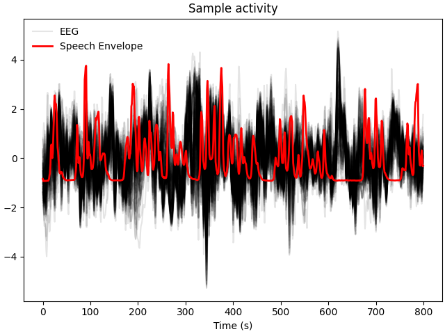
首先加载 [1] 中采集的数据。该实验中被试聆听自然语音，提供原始 EEG 与语音刺激。下面加载数据并降采样以加快计算，因为已知特征主要为低频。随后可视化 EEG 与语音包络。

path = mne.datasets.mtrf.data_path()
decim = 2
data = loadmat(join(path, "speech_data.mat"))
raw = data["EEG"].T
speech = data["envelope"].T
sfreq = float(data["Fs"].item())
sfreq /= decim
speech = mne.filter.resample(speech, down=decim, method="polyphase")
raw = mne.filter.resample(raw, down=decim, method="polyphase")

# Read in channel positions and create our MNE objects from the raw data
montage = mne.channels.make_standard_montage("biosemi128")
info = mne.create_info(montage.ch_names, sfreq, "eeg").set_montage(montage)
raw = mne.io.RawArray(raw, info)
n_channels = len(raw.ch_names)

# Plot a sample of brain and stimulus activity
fig, ax = plt.subplots(layout="constrained")
lns = ax.plot(scale(raw[:, :800][0].T), color="k", alpha=0.1)
ln1 = ax.plot(scale(speech[0, :800]), color="r", lw=2)
ax.legend([lns[0], ln1[0]], ["EEG", "Speech Envelope"], frameon=False)
ax.set(title="Sample activity", xlabel="Time (s)")

Polyphase resampling neighborhood: ±2 input samples
Polyphase resampling neighborhood: ±2 input samples
Creating RawArray with float64 data, n_channels=128, n_times=7677
    Range : 0 ... 7676 =      0.000 ...   119.938 secs
Ready.

创建并拟合感受野模型#

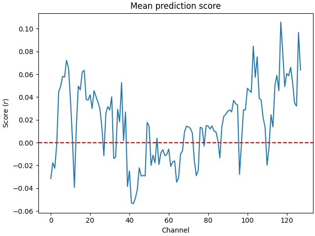
我们构建编码模型，找出语音包络的时间延迟版本与 EEG 信号之间的线性关系，从而可对新刺激的响应做出预测。

# Define the delays that we will use in the receptive field
tmin, tmax = -0.2, 0.4

# Initialize the model
rf = ReceptiveField(
    tmin, tmax, sfreq, feature_names=["envelope"], estimator=1.0, scoring="corrcoef"
)
# We'll have (tmax - tmin) * sfreq delays
# and an extra 2 delays since we are inclusive on the beginning / end index
n_delays = int((tmax - tmin) * sfreq) + 2

n_splits = 3
cv = KFold(n_splits)

# Prepare model data (make time the first dimension)
speech = speech.T
Y, _ = raw[:]  # Outputs for the model
Y = Y.T

# Iterate through splits, fit the model, and predict/test on held-out data
coefs = np.zeros((n_splits, n_channels, n_delays))
scores = np.zeros((n_splits, n_channels))
for ii, (train, test) in enumerate(cv.split(speech)):
    print(f"split {ii + 1} / {n_splits}")
    rf.fit(speech[train], Y[train])
    scores[ii] = rf.score(speech[test], Y[test])
    # coef_ is shape (n_outputs, n_features, n_delays). we only have 1 feature
    coefs[ii] = rf.coef_[:, 0, :]
times = rf.delays_ / float(rf.sfreq)

# Average scores and coefficients across CV splits
mean_coefs = coefs.mean(axis=0)
mean_scores = scores.mean(axis=0)

# Plot mean prediction scores across all channels
fig, ax = plt.subplots(layout="constrained")
ix_chs = np.arange(n_channels)
ax.plot(ix_chs, mean_scores)
ax.axhline(0, ls="--", color="r")
ax.set(title="Mean prediction score", xlabel="Channel", ylabel="Score ($r$)")

split 1 / 3
Fitting 1 epochs, 1 channels

  0%|          | Sample : 0/2 [00:00<?,       ?it/s]
 50%|█████     | Sample : 1/2 [00:02<00:02,    2.20s/it]split 2 / 3
Fitting 1 epochs, 1 channels


  0%|          | Sample : 0/2 [00:00<?,       ?it/s]

100%|██████████| Sample : 2/2 [00:00<00:00,  110.87it/s]
100%|██████████| Sample : 2/2 [00:00<00:00,  109.42it/s]
split 3 / 3
Fitting 1 epochs, 1 channels


  0%|          | Sample : 0/2 [00:00<?,       ?it/s]
100%|██████████| Sample : 2/2 [00:00<00:00,  149.35it/s]

研究模型系数#

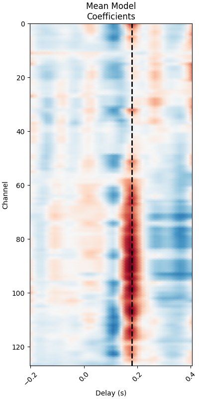
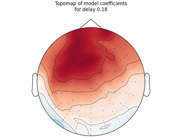
最后查看线性系数（有时称为 beta 值）在时间延迟与头皮上的分布，复现 [1] 的图 1 与图 2。

# Print mean coefficients across all time delays / channels (see Fig 1)
time_plot = 0.180  # For highlighting a specific time.
fig, ax = plt.subplots(figsize=(4, 8), layout="constrained")
max_coef = mean_coefs.max()
ax.pcolormesh(
    times,
    ix_chs,
    mean_coefs,
    cmap="RdBu_r",
    vmin=-max_coef,
    vmax=max_coef,
    shading="gouraud",
)
ax.axvline(time_plot, ls="--", color="k", lw=2)
ax.set(
    xlabel="Delay (s)",
    ylabel="Channel",
    title="Mean Model\nCoefficients",
    xlim=times[[0, -1]],
    ylim=[len(ix_chs) - 1, 0],
    xticks=np.arange(tmin, tmax + 0.2, 0.2),
)
plt.setp(ax.get_xticklabels(), rotation=45)

# Make a topographic map of coefficients for a given delay (see Fig 2C)
ix_plot = np.argmin(np.abs(time_plot - times))
fig, ax = plt.subplots(layout="constrained")
mne.viz.plot_topomap(
    mean_coefs[:, ix_plot], pos=info, axes=ax, show=False, vlim=(-max_coef, max_coef)
)
ax.set(title=f"Topomap of model coefficients\nfor delay {time_plot}")

创建并拟合刺激重建模型#

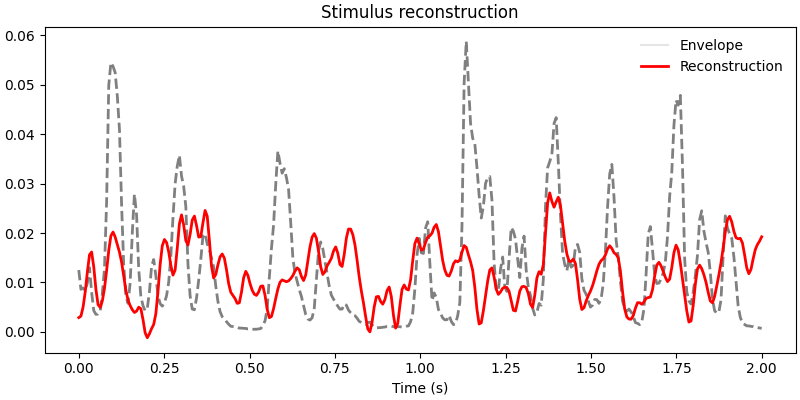
下面演示 mne.decoding.ReceptiveField 类的另一个用途：从 EEG 数据预测刺激活动。文献中称为解码模型或刺激重建模型 [1]。解码模型旨在找出语音信号与 EEG 时间延迟版本之间的关系。与把每个 M/EEG 通道视为独立特征的编码情形相比，它能在多变量框架中利用全部神经数据，因此对语音这类低信噪比刺激可能拟合得更好（代价是未控制刺激协方差）。

# We use the same lags as in :footcite:`CrosseEtAl2016`. Negative lags now
# index the relationship
# between the neural response and the speech envelope earlier in time, whereas
# positive lags would index how a unit change in the amplitude of the EEG would
# affect later stimulus activity (obviously this should have an amplitude of
# zero).
tmin, tmax = -0.2, 0.0

# Initialize the model. Here the features are the EEG data. We also specify
# ``patterns=True`` to compute inverse-transformed coefficients during model
# fitting (cf. next section and :footcite:`HaufeEtAl2014`).
# We'll use a ridge regression estimator with an alpha value similar to
# Crosse et al.
sr = ReceptiveField(
    tmin,
    tmax,
    sfreq,
    feature_names=raw.ch_names,
    estimator=1e4,
    scoring="corrcoef",
    patterns=True,
)
# We'll have (tmax - tmin) * sfreq delays
# and an extra 2 delays since we are inclusive on the beginning / end index
n_delays = int((tmax - tmin) * sfreq) + 2

n_splits = 3
cv = KFold(n_splits)

# Iterate through splits, fit the model, and predict/test on held-out data
coefs = np.zeros((n_splits, n_channels, n_delays))
patterns = coefs.copy()
scores = np.zeros((n_splits,))
for ii, (train, test) in enumerate(cv.split(speech)):
    print(f"split {ii + 1} / {n_splits}")
    sr.fit(Y[train], speech[train])
    scores[ii] = sr.score(Y[test], speech[test])[0]
    # coef_ is shape (n_outputs, n_features, n_delays). We have 128 features
    coefs[ii] = sr.coef_[0, :, :]
    patterns[ii] = sr.patterns_[0, :, :]
times = sr.delays_ / float(sr.sfreq)

# Average scores and coefficients across CV splits
mean_coefs = coefs.mean(axis=0)
mean_patterns = patterns.mean(axis=0)
mean_scores = scores.mean(axis=0)
max_coef = np.abs(mean_coefs).max()
max_patterns = np.abs(mean_patterns).max()

split 1 / 3
Fitting 1 epochs, 128 channels

  0%|          | Sample : 0/8384 [00:00<?,       ?it/s]

  2%|▏         | Sample : 171/8384 [00:00<00:00, 10670.94it/s]

  6%|▌         | Sample : 473/8384 [00:00<00:00, 14856.01it/s]

  9%|▉         | Sample : 778/8384 [00:00<00:00, 16311.28it/s]

 13%|█▎        | Sample : 1084/8384 [00:00<00:00, 17061.00it/s]

 17%|█▋        | Sample : 1390/8384 [00:00<00:00, 17505.19it/s]

 20%|██        | Sample : 1696/8384 [00:00<00:00, 17806.18it/s]

 24%|██▍       | Sample : 2004/8384 [00:00<00:00, 18035.81it/s]

 28%|██▊       | Sample : 2311/8384 [00:00<00:00, 18204.39it/s]

 31%|███       | Sample : 2619/8384 [00:00<00:00, 18339.96it/s]

 35%|███▍      | Sample : 2926/8384 [00:00<00:00, 18441.20it/s]

 39%|███▊      | Sample : 3232/8384 [00:00<00:00, 18515.29it/s]

 42%|████▏     | Sample : 3538/8384 [00:00<00:00, 18578.72it/s]

 46%|████▌     | Sample : 3845/8384 [00:00<00:00, 18637.74it/s]

 50%|████▉     | Sample : 4151/8384 [00:00<00:00, 18679.91it/s]

 53%|█████▎    | Sample : 4455/8384 [00:00<00:00, 18709.57it/s]

 57%|█████▋    | Sample : 4738/8384 [00:00<00:00, 18616.81it/s]

 60%|█████▉    | Sample : 5024/8384 [00:00<00:00, 18552.27it/s]

 64%|██████▎   | Sample : 5332/8384 [00:00<00:00, 18606.29it/s]

 67%|██████▋   | Sample : 5640/8384 [00:00<00:00, 18656.62it/s]

 71%|███████   | Sample : 5948/8384 [00:00<00:00, 18700.63it/s]

 75%|███████▍  | Sample : 6255/8384 [00:00<00:00, 18735.28it/s]

 78%|███████▊  | Sample : 6562/8384 [00:00<00:00, 18766.08it/s]

 82%|████████▏ | Sample : 6868/8384 [00:00<00:00, 18789.58it/s]

 86%|████████▌ | Sample : 7174/8384 [00:00<00:00, 18812.73it/s]

 89%|████████▉ | Sample : 7481/8384 [00:00<00:00, 18835.77it/s]

 93%|█████████▎| Sample : 7787/8384 [00:00<00:00, 18853.53it/s]

 97%|█████████▋| Sample : 8091/8384 [00:00<00:00, 18863.24it/s]

100%|█████████▉| Sample : 8382/8384 [00:00<00:00, 18817.84it/s]
100%|██████████| Sample : 8384/8384 [00:00<00:00, 18675.60it/s]
split 2 / 3
Fitting 1 epochs, 128 channels

  0%|          | Sample : 0/8384 [00:00<?,       ?it/s]

  2%|▏         | Sample : 135/8384 [00:00<00:00, 8411.16it/s]

  5%|▌         | Sample : 434/8384 [00:00<00:00, 13650.96it/s]

  9%|▉         | Sample : 737/8384 [00:00<00:00, 15495.22it/s]

 12%|█▏        | Sample : 1043/8384 [00:00<00:00, 16458.13it/s]

 16%|█▌        | Sample : 1350/8384 [00:00<00:00, 17052.60it/s]

 20%|█▉        | Sample : 1659/8384 [00:00<00:00, 17471.38it/s]

 23%|██▎       | Sample : 1966/8384 [00:00<00:00, 17750.87it/s]

 27%|██▋       | Sample : 2275/8384 [00:00<00:00, 17974.94it/s]

 31%|███       | Sample : 2583/8384 [00:00<00:00, 18141.76it/s]

 34%|███▍      | Sample : 2889/8384 [00:00<00:00, 18260.61it/s]

 38%|███▊      | Sample : 3196/8384 [00:00<00:00, 18360.97it/s]

 42%|████▏     | Sample : 3502/8384 [00:00<00:00, 18438.09it/s]

 45%|████▌     | Sample : 3810/8384 [00:00<00:00, 18521.19it/s]

 49%|████▉     | Sample : 4116/8384 [00:00<00:00, 18579.16it/s]

 53%|█████▎    | Sample : 4421/8384 [00:00<00:00, 18621.63it/s]

 56%|█████▌    | Sample : 4707/8384 [00:00<00:00, 18553.90it/s]

 60%|█████▉    | Sample : 4989/8384 [00:00<00:00, 18469.85it/s]

 63%|██████▎   | Sample : 5298/8384 [00:00<00:00, 18535.14it/s]

 67%|██████▋   | Sample : 5606/8384 [00:00<00:00, 18588.44it/s]

 71%|███████   | Sample : 5913/8384 [00:00<00:00, 18634.35it/s]

 74%|███████▍  | Sample : 6220/8384 [00:00<00:00, 18672.76it/s]

 78%|███████▊  | Sample : 6524/8384 [00:00<00:00, 18692.60it/s]

 81%|████████▏ | Sample : 6829/8384 [00:00<00:00, 18717.38it/s]

 85%|████████▌ | Sample : 7133/8384 [00:00<00:00, 18736.16it/s]

 89%|████████▊ | Sample : 7438/8384 [00:00<00:00, 18755.45it/s]

 92%|█████████▏| Sample : 7743/8384 [00:00<00:00, 18773.04it/s]

 96%|█████████▌| Sample : 8046/8384 [00:00<00:00, 18780.59it/s]

 99%|█████████▉| Sample : 8341/8384 [00:00<00:00, 18755.31it/s]
100%|██████████| Sample : 8384/8384 [00:00<00:00, 18573.92it/s]
split 3 / 3
Fitting 1 epochs, 128 channels

  0%|          | Sample : 0/8384 [00:00<?,       ?it/s]

  2%|▏         | Sample : 134/8384 [00:00<00:00, 8371.86it/s]

  5%|▌         | Sample : 428/8384 [00:00<00:00, 13486.71it/s]

  9%|▊         | Sample : 732/8384 [00:00<00:00, 15403.41it/s]

 12%|█▏        | Sample : 1027/8384 [00:00<00:00, 16206.74it/s]

 16%|█▌        | Sample : 1324/8384 [00:00<00:00, 16722.99it/s]

 19%|█▉        | Sample : 1621/8384 [00:00<00:00, 17068.65it/s]

 23%|██▎       | Sample : 1919/8384 [00:00<00:00, 17318.63it/s]

 26%|██▋       | Sample : 2218/8384 [00:00<00:00, 17516.06it/s]

 30%|███       | Sample : 2518/8384 [00:00<00:00, 17678.17it/s]

 34%|███▎      | Sample : 2820/8384 [00:00<00:00, 17822.97it/s]

 37%|███▋      | Sample : 3125/8384 [00:00<00:00, 17961.04it/s]

 41%|████      | Sample : 3428/8384 [00:00<00:00, 18066.72it/s]

 45%|████▍     | Sample : 3733/8384 [00:00<00:00, 18167.04it/s]

 48%|████▊     | Sample : 4037/8384 [00:00<00:00, 18245.74it/s]

 52%|█████▏    | Sample : 4341/8384 [00:00<00:00, 18315.50it/s]

 55%|█████▌    | Sample : 4636/8384 [00:00<00:00, 18325.62it/s]

 59%|█████▊    | Sample : 4907/8384 [00:00<00:00, 18205.74it/s]

 62%|██████▏   | Sample : 5214/8384 [00:00<00:00, 18286.20it/s]

 66%|██████▌   | Sample : 5522/8384 [00:00<00:00, 18358.85it/s]

 70%|██████▉   | Sample : 5830/8384 [00:00<00:00, 18426.24it/s]

 73%|███████▎  | Sample : 6136/8384 [00:00<00:00, 18475.42it/s]

 77%|███████▋  | Sample : 6438/8384 [00:00<00:00, 18503.04it/s]

 80%|████████  | Sample : 6743/8384 [00:00<00:00, 18539.21it/s]

 84%|████████▍ | Sample : 7047/8384 [00:00<00:00, 18569.35it/s]

 88%|████████▊ | Sample : 7351/8384 [00:00<00:00, 18596.94it/s]

 91%|█████████▏| Sample : 7657/8384 [00:00<00:00, 18631.61it/s]

 95%|█████████▍| Sample : 7963/8384 [00:00<00:00, 18661.00it/s]

 98%|█████████▊| Sample : 8258/8384 [00:00<00:00, 18642.94it/s]
100%|██████████| Sample : 8384/8384 [00:00<00:00, 18403.38it/s]

可视化刺激重建#

为直观了解模型性能，可并排绘制真实与预测的刺激包络。

y_pred = sr.predict(Y[test])
time = np.linspace(0, 2.0, 5 * int(sfreq))
fig, ax = plt.subplots(figsize=(8, 4), layout="constrained")
ax.plot(
    time, speech[test][sr.valid_samples_][: int(5 * sfreq)], color="grey", lw=2, ls="--"
)
ax.plot(time, y_pred[sr.valid_samples_][: int(5 * sfreq)], color="r", lw=2)
ax.legend([lns[0], ln1[0]], ["Envelope", "Reconstruction"], frameon=False)
ax.set(title="Stimulus reconstruction")
ax.set_xlabel("Time (s)")

研究模型系数#

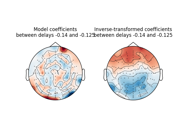
最后查看解码模型系数在头皮上的分布，尝试复现 [1] 的图 5。解码模型权重反映对重建刺激信号贡献最大的通道，但无法从神经生理角度直接解释。这里还查看通过反演过程得到的系数 [2]，其数值（与符号）直接对应刺激信号的强度（与效应方向），解释更直接。

time_plot = (-0.140, -0.125)  # To average between two timepoints.
ix_plot = np.arange(
    np.argmin(np.abs(time_plot[0] - times)), np.argmin(np.abs(time_plot[1] - times))
)
fig, ax = plt.subplots(1, 2)
mne.viz.plot_topomap(
    np.mean(mean_coefs[:, ix_plot], axis=1),
    pos=info,
    axes=ax[0],
    show=False,
    vlim=(-max_coef, max_coef),
)
ax[0].set(title=f"Model coefficients\nbetween delays {time_plot[0]} and {time_plot[1]}")

mne.viz.plot_topomap(
    np.mean(mean_patterns[:, ix_plot], axis=1),
    pos=info,
    axes=ax[1],
    show=False,
    vlim=(-max_patterns, max_patterns),
)
ax[1].set(
    title=(
        f"Inverse-transformed coefficients\nbetween delays {time_plot[0]} and "
        f"{time_plot[1]}"
    )
)

Model coefficients between delays -0.14 and -0.125, Inverse-transformed coefficients between delays -0.14 and -0.125

参考文献#

脚本总运行时间：（0 分 6.998 秒）

图库由 Sphinx-Gallery 生成