
说明
转到末尾下载完整示例代码。
计算协方差矩阵#
MNE 中的许多方法,包括源估计和部分分类算法,都需要基于记录数据估计协方差。本教程介绍传感器协方差计算的基础知识,并构建一个可用于计算最小范数逆解的噪声协方差矩阵。更多信息参见 The minimum-norm current estimates。
# Authors: The MNE-Python contributors.
# License: BSD-3-Clause
# Copyright the MNE-Python contributors.
import mne
from mne.datasets import sample
MNE 等源估计方法需要基于记录数据估计噪声。本教程介绍噪声协方差的基础知识,并构建一个可用于计算逆解的噪声协方差矩阵。更多信息参见 The minimum-norm current estimates。
data_path = sample.data_path()
raw_empty_room_fname = data_path / "MEG" / "sample" / "ernoise_raw.fif"
raw_empty_room = mne.io.read_raw_fif(raw_empty_room_fname)
raw_fname = data_path / "MEG" / "sample" / "sample_audvis_raw.fif"
raw = mne.io.read_raw_fif(raw_fname)
raw.set_eeg_reference("average", projection=True)
raw.info["bads"] += ["EEG 053"]  # bads + 1 more
Opening raw data file /home/circleci/mne_data/MNE-sample-data/MEG/sample/ernoise_raw.fif...
Isotrak not found
    Read a total of 3 projection items:
        PCA-v1 (1 x 10²)  idle
        PCA-v2 (1 x 10²)  idle
        PCA-v3 (1 x 10²)  idle
    Range : 19800 ... 85867 =     32.966 ...   142.965 secs
Ready.
Opening raw data file /home/circleci/mne_data/MNE-sample-data/MEG/sample/sample_audvis_raw.fif...
    Read a total of 3 projection items:
        PCA-v1 (1 x 10²)  idle
        PCA-v2 (1 x 10²)  idle
        PCA-v3 (1 x 10²)  idle
    Range : 25800 ... 192599 =     42.956 ...   320.670 secs
Ready.
EEG channel type selected for re-referencing
Adding average EEG reference projection.
1 projection items deactivated
噪声的定义取决于实验范式。在 MEG 中,常用空房间测量来估计传感器噪声。不过,如果你处理的是诱发响应,可能还需要把静息态脑活动也视为噪声。首先,我们用空房间记录计算噪声。注意,你也可以通过 tmin 和 tmax 参数只使用记录的一部分,这在把静息态作为噪声基线时很有用。这里我们使用整段空房间记录来计算噪声协方差(tmax=None 等同于记录结束,见 mne.compute_raw_covariance())。
请记住,在处理流程上要让空房间数据集与实际 MEG 数据相匹配。确保滤波器完全相同;如果使用 ICA,也要对空房间数据和受试者数据做同等处理。本例中我们没有对数据滤波,也没有使用 ICA。不过,MEG 数据中确实存在坏导和投影,因此我们需要确保它们被保存到协方差对象中。
raw_empty_room.info["bads"] = [bb for bb in raw.info["bads"] if "EEG" not in bb]
raw_empty_room.add_proj(
    [pp.copy() for pp in raw.info["projs"] if "EEG" not in pp["desc"]]
)

noise_cov = mne.compute_raw_covariance(raw_empty_room, tmin=0, tmax=None)
3 projection items deactivated
Using up to 550 segments
Number of samples used : 66000
[done]
现在协方差矩阵已保存在 MNE-Python 对象中,你可以用 mne.write_cov() 将其保存到文件,之后再用 mne.read_cov() 读回。
你也可以用刺激前基线来估计噪声协方差。首先需要构建 epochs。计算协方差时,应在构建 epochs 时进行基线校正,否则协方差矩阵会不准确。在 MNE 中这是默认行为,但为确保无误,我们在这里手动指定。
events = mne.find_events(raw)
epochs = mne.Epochs(
    raw,
    events,
    event_id=1,
    tmin=-0.2,
    tmax=0.5,
    baseline=(-0.2, 0.0),
    decim=3,  # we'll decimate for speed
    verbose="error",
)  # and ignore the warning about aliasing
Finding events on: STI 014
320 events found on stim channel STI 014
Event IDs: [ 1  2  3  4  5 32]
注意,无论你是否愿意,这种方法还会削弱源估计中任何与基线相似的活动。
noise_cov_baseline = mne.compute_covariance(epochs, tmax=0)
Loading data for 72 events and 421 original time points (prior to decimation) ...
0 bad epochs dropped
    Created an SSP operator (subspace dimension = 4)
    Setting small MEG eigenvalues to zero (without PCA)
    Setting small EEG eigenvalues to zero (without PCA)
Reducing data rank from 364 -> 360
Estimating covariance using EMPIRICAL
Done.
Number of samples used : 2952
[done]
绘制协方差矩阵#
可以尝试将 proj 设为 False 来观察效果。注意,epochs 中的投影器已经应用,因此 proj 参数不会产生作用。
noise_cov.plot(raw_empty_room.info, proj=True)
noise_cov_baseline.plot(epochs.info, proj=True)
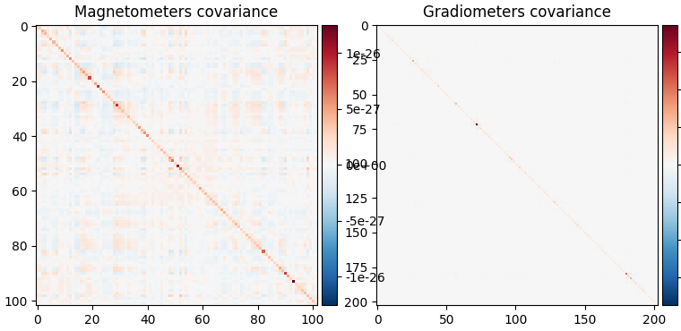
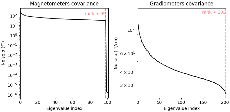
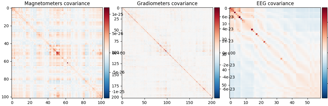
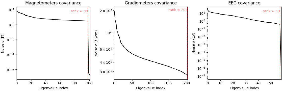
    Created an SSP operator (subspace dimension = 3)
Computing rank from covariance with rank=None
    Using tolerance 1.2e-15 (2.2e-16 eps * 102 dim * 0.052  max singular value)
    Estimated rank (mag): 99
    MAG: rank 99 computed from 102 data channels with 0 projectors
Computing rank from covariance with rank=None
    Using tolerance 9.7e-14 (2.2e-16 eps * 203 dim * 2.2  max singular value)
    Estimated rank (grad): 203
    GRAD: rank 203 computed from 203 data channels with 0 projectors
    Created an SSP operator (subspace dimension = 4)
Computing rank from covariance with rank=None
    Using tolerance 2.2e-14 (2.2e-16 eps * 102 dim * 0.96  max singular value)
    Estimated rank (mag): 99
    MAG: rank 99 computed from 102 data channels with 0 projectors
Computing rank from covariance with rank=None
    Using tolerance 1.9e-13 (2.2e-16 eps * 203 dim * 4.1  max singular value)
    Estimated rank (grad): 203
    GRAD: rank 203 computed from 203 data channels with 0 projectors
Computing rank from covariance with rank=None
    Using tolerance 8.4e-14 (2.2e-16 eps * 59 dim * 6.4  max singular value)
    Estimated rank (eeg): 58
    EEG: rank 58 computed from 59 data channels with 0 projectors
如何对协方差矩阵进行正则化?#
估计得到的协方差在数值上可能不稳定,并且容易使估计的源幅值与可用样本数之间产生相关性。因此 MNE 手册建议对噪声协方差矩阵进行正则化(参见 Regularization of the noise-covariance matrix),尤其是在样本很少时。遗憾的是,有效样本数并不容易确定,因此也难以选择合适的正则化强度。在 MNE-Python 中,正则化通过 Engemann 和 Gramfort [1] 所述的先进正则化方法完成。为此可以使用 'auto' 选项;启用该选项后,将通过交叉验证学习最优正则化参数:
noise_cov_reg = mne.compute_covariance(epochs, tmax=0.0, method="auto", rank=None)
Loading data for 72 events and 421 original time points (prior to decimation) ...
    Created an SSP operator (subspace dimension = 4)
    Setting small MEG eigenvalues to zero (without PCA)
    Setting small EEG eigenvalues to zero (without PCA)
Reducing data rank from 364 -> 360
Estimating covariance using SHRUNK
Done.
Estimating covariance using DIAGONAL_FIXED
    MAG regularization : 0.1
    GRAD regularization : 0.1
    EEG regularization : 0.1
Done.
Estimating covariance using EMPIRICAL
Done.
Using cross-validation to select the best estimator.
    MAG regularization : 0.1
    GRAD regularization : 0.1
    EEG regularization : 0.1
    MAG regularization : 0.1
    GRAD regularization : 0.1
    EEG regularization : 0.1
    MAG regularization : 0.1
    GRAD regularization : 0.1
    EEG regularization : 0.1
Number of samples used : 2952
log-likelihood on unseen data (descending order):
   shrunk: -1768.715
   diagonal_fixed: -1785.397
   empirical: -1797.005
selecting best estimator: shrunk
[done]
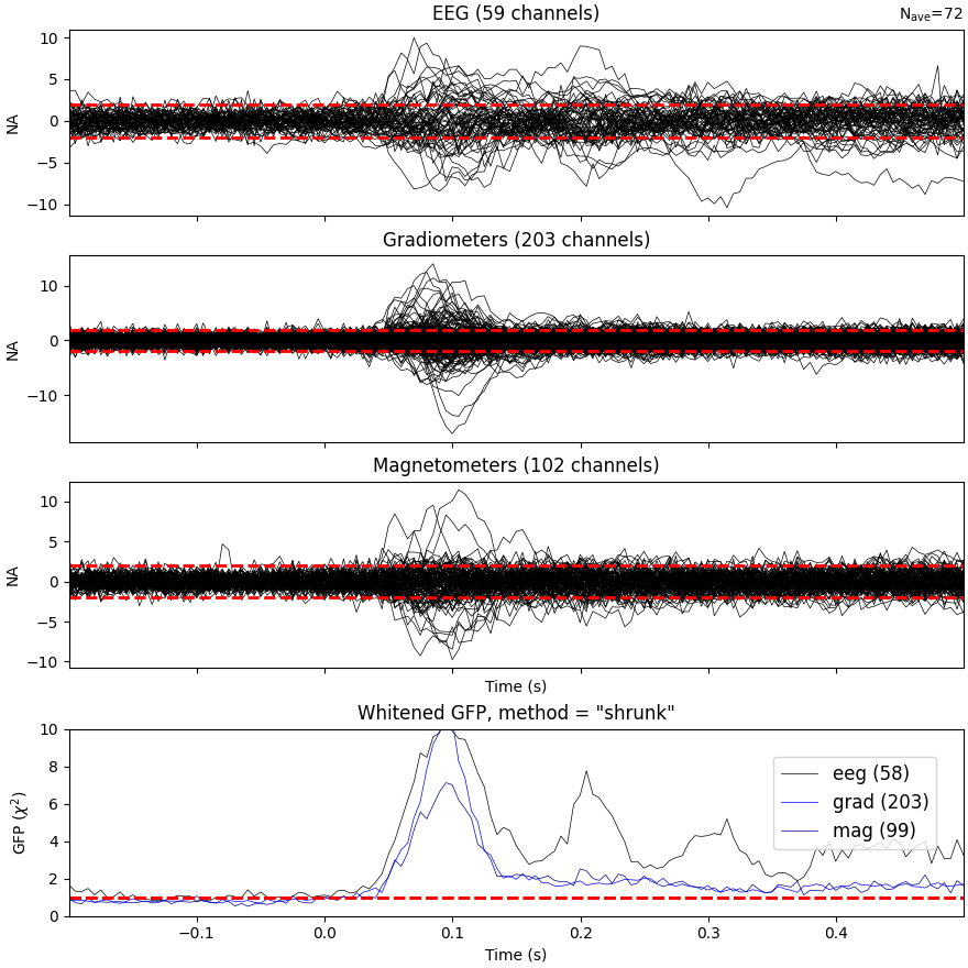
该过程利用未见数据的负对数似然,根据白化数据的程度定量评估噪声协方差。最终结果也可以进行可视化检查。假设基线中不含系统性信号(与感兴趣事件锁时),白化后的基线信号应服从多元高斯分布,即在给定时间采样点上,白化基线信号应位于 -1.96 与 1.96 之间。基于同样的推理,全局场功率(global field power,GFP)的期望值为 1(计算 GFP 时应考虑真实自由度,例如有 2 个激活的 SSP 向量时取 ddof=3):
evoked = epochs.average()
evoked.plot_white(noise_cov_reg, time_unit="s")
NOTE: pick_types() is a legacy function. New code should use inst.pick(...).
Computing rank from covariance with rank=None
    Using tolerance 8.4e-14 (2.2e-16 eps * 59 dim * 6.4  max singular value)
    Estimated rank (eeg): 58
    EEG: rank 58 computed from 59 data channels with 1 projector
Computing rank from covariance with rank=None
    Using tolerance 1.8e-13 (2.2e-16 eps * 203 dim * 4  max singular value)
    Estimated rank (grad): 203
    GRAD: rank 203 computed from 203 data channels with 0 projectors
Computing rank from covariance with rank=None
    Using tolerance 2.1e-14 (2.2e-16 eps * 102 dim * 0.91  max singular value)
    Estimated rank (mag): 99
    MAG: rank 99 computed from 102 data channels with 3 projectors
    Created an SSP operator (subspace dimension = 4)
Computing rank from covariance with rank={'eeg': 58, 'grad': 203, 'mag': 99, 'meg': 302}
    Setting small MEG eigenvalues to zero (without PCA)
    Setting small EEG eigenvalues to zero (without PCA)
    Created the whitener using a noise covariance matrix with rank 360 (4 small eigenvalues omitted)
该图同时显示各通道的白化诱发信号和白化 GFP。GFP 面板中的数字表示数据的估计秩,即在计算白化 GFP 时,用于除以跨传感器平方和的等效自由度。白化 GFP 还有助于检测虚假的晚期诱发成分,这类成分可能是正则化过度或不足的结果。
注意,如果数据已使用信号空间分离(signal space separation,SSS)[2] 处理,梯度计和磁力计将联合显示,因为二者都是由相同的 SSS 基向量重建的,具有相同的数值秩。这也意味着这两种传感器类型不再在统计上独立。这些评估方法可用于检验模型违背情况。更多入门材料可参见此处。
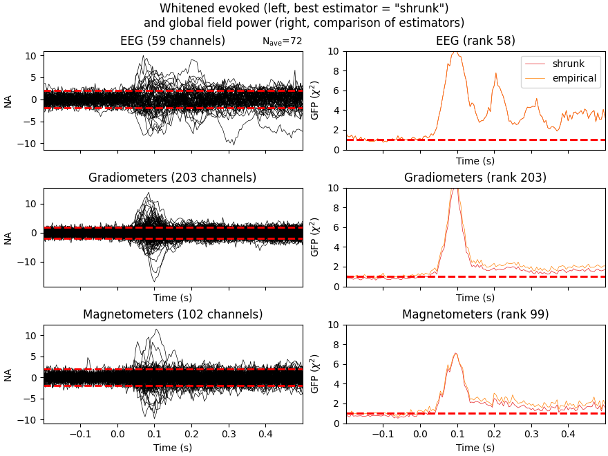
对于高级用法或调试,还可以比较不同的替代估计器(参见 Whitening evoked data with a noise covariance):
noise_covs = mne.compute_covariance(
    epochs, tmax=0.0, method=("empirical", "shrunk"), return_estimators=True, rank=None
)
evoked.plot_white(noise_covs, time_unit="s")
Loading data for 72 events and 421 original time points (prior to decimation) ...
    Created an SSP operator (subspace dimension = 4)
    Setting small MEG eigenvalues to zero (without PCA)
    Setting small EEG eigenvalues to zero (without PCA)
Reducing data rank from 364 -> 360
Estimating covariance using EMPIRICAL
Done.
Estimating covariance using SHRUNK
Done.
Using cross-validation to select the best estimator.
Number of samples used : 2952
log-likelihood on unseen data (descending order):
   shrunk: -1768.715
   empirical: -1797.005
[done]
NOTE: pick_types() is a legacy function. New code should use inst.pick(...).
Computing rank from covariance with rank=None
    Using tolerance 8.4e-14 (2.2e-16 eps * 59 dim * 6.4  max singular value)
    Estimated rank (eeg): 58
    EEG: rank 58 computed from 59 data channels with 1 projector
Computing rank from covariance with rank=None
    Using tolerance 1.8e-13 (2.2e-16 eps * 203 dim * 4  max singular value)
    Estimated rank (grad): 203
    GRAD: rank 203 computed from 203 data channels with 0 projectors
Computing rank from covariance with rank=None
    Using tolerance 2.1e-14 (2.2e-16 eps * 102 dim * 0.91  max singular value)
    Estimated rank (mag): 99
    MAG: rank 99 computed from 102 data channels with 3 projectors
Computing rank from covariance with rank=None
    Using tolerance 8.4e-14 (2.2e-16 eps * 59 dim * 6.4  max singular value)
    Estimated rank (eeg): 58
    EEG: rank 58 computed from 59 data channels with 1 projector
Computing rank from covariance with rank=None
    Using tolerance 1.9e-13 (2.2e-16 eps * 203 dim * 4.1  max singular value)
    Estimated rank (grad): 203
    GRAD: rank 203 computed from 203 data channels with 0 projectors
Computing rank from covariance with rank=None
    Using tolerance 2.2e-14 (2.2e-16 eps * 102 dim * 0.96  max singular value)
    Estimated rank (mag): 99
    MAG: rank 99 computed from 102 data channels with 3 projectors
    Created an SSP operator (subspace dimension = 4)
Computing rank from covariance with rank={'eeg': 58, 'grad': 203, 'mag': 99, 'meg': 302}
    Setting small MEG eigenvalues to zero (without PCA)
    Setting small EEG eigenvalues to zero (without PCA)
    Created the whitener using a noise covariance matrix with rank 360 (4 small eigenvalues omitted)
这将绘制最优估计器的白化诱发数据,并在相应面板中以独立线条显示所有估计器的 GFP。
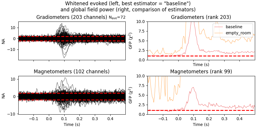
最后,我们来看空房间协方差与事件相关协方差之间的差异,通过 hack "method" 选项,让二者的类型显示在图的图例中。
evoked_meg = evoked.copy().pick("meg")
noise_cov["method"] = "empty_room"
noise_cov_baseline["method"] = "baseline"
evoked_meg.plot_white([noise_cov_baseline, noise_cov], time_unit="s")
NOTE: pick_types() is a legacy function. New code should use inst.pick(...).
Computing rank from covariance with rank=None
    Using tolerance 1.9e-13 (2.2e-16 eps * 203 dim * 4.1  max singular value)
    Estimated rank (grad): 203
    GRAD: rank 203 computed from 203 data channels with 0 projectors
Computing rank from covariance with rank=None
    Using tolerance 2.2e-14 (2.2e-16 eps * 102 dim * 0.96  max singular value)
    Estimated rank (mag): 99
    MAG: rank 99 computed from 102 data channels with 3 projectors
Computing rank from covariance with rank=None
    Using tolerance 9.7e-14 (2.2e-16 eps * 203 dim * 2.2  max singular value)
    Estimated rank (grad): 203
    GRAD: rank 203 computed from 203 data channels with 0 projectors
Computing rank from covariance with rank=None
    Using tolerance 1.2e-15 (2.2e-16 eps * 102 dim * 0.052  max singular value)
    Estimated rank (mag): 99
    MAG: rank 99 computed from 102 data channels with 3 projectors
    Created an SSP operator (subspace dimension = 3)
Computing rank from covariance with rank={'grad': 203, 'mag': 99, 'meg': 302}
    Setting small MEG eigenvalues to zero (without PCA)
    Created the whitener using a noise covariance matrix with rank 302 (3 small eigenvalues omitted)
    Created an SSP operator (subspace dimension = 3)
Computing rank from covariance with rank={'grad': 203, 'mag': 99, 'meg': 302}
    Setting small MEG eigenvalues to zero (without PCA)
    Created the whitener using a noise covariance matrix with rank 302 (3 small eigenvalues omitted)
根据负对数似然,基线协方差似乎更合适。不恰当的正则化可能导致源幅值被高估,更多信息和示例参见 [1]。
参考文献#
脚本总运行时间:(0 分 11.290 秒)